Author(s): Xiaolin Hu is a second-year PhD student at the Gaoling School of Artificial Intelligence, Renmin University of China. He is working on deep learning theory and AI4Science with Prof. Yong Liu. Recently, he has been particularly interested in exploring the interaction between deep learning and dynamic systems. Xiaolin obtained his Bachelor’s and Master’s degrees in Communication and Information System from Shanghai University (SHU) in 2018 and 2021, respectively. During his time at SHU, he worked on developing intelligent communication systems under the supervision of Prof. Nicholas E. Buris.
Introduction
Over the past 10 years, deep learning models achieve great success in different fields, including computer vision, neural language processing, and recommendation system. The objective of the training is to output a model that correctly labels training examples. In practice, the trained model will be applied to predict labels of unseen examples. For instance, the models used in automated driving should have the ability to detect obstacles that are not included in training examples. A model’s ability to label unseen examples is called generalization. One commonly used method to approximate generalization error is to keep some test examples and then measure the distance between the predicted labels and true labels. In this section, we use statistical tools to analyze the generalization of deep learning models theoretically.
Generalization is the Goal of Learning
Machine learning is widely used to solve problems that can not be programmed directly. All machine learning problems involve some core components:
- The data that we can learn from.
- A output model trained from data.
- A algorithm to train the model.
The fundamental question is how to measure the performance of the trained model. To answer this question, we first need to ask the following question:
- What is the goal of learning?
In the training phase, an optimization algorithm like stochastic gradient descent (SGD) is applied to adjust the model to fit the training data. Therefore, the output model is affected by the training algorithm and training data. In specific, the performance of the model during training can be measured by the distance between labels predicted by the model and the true labels of training data. This distance is quantified by an objective function (loss function).
The goal of training is to output a model fitting the training (seen) examples well. However, what we care about is the model’s ability to label unseen examples. Thus, the goal of learning is to output a model fitting the unseen testing examples well. In summary, generalization performance reflects the model’s ability to label unseen testing data. Optimization performance reflects the model’s ability to label seen training data. Therefore, understanding generalization is the most fundamental task in machine learning theory. In this chapter, we focus on understanding the generalization of deep learning models.
Let’s start with a simple example. Suppose we have a coin with unknown probability \(\theta\) of heads. We hope to estimate this unknown probability \(\theta\) by experiments of repeat tossing. Let \(X\) denote the random output of one toss where \(X=1\) if head and \(X=0\) if tail. If we toss the coin \(n\) times independently, the experimental outcome of \(i\)-th coin toss, \(X_i\), is independent of all other outcomes. It is clear that each \(X_i \in \{ 0,1 \}\) and \(\mathbb{P}(X_i = 1) = \theta.\) We denote the sequence of outcomes by \(X^n = \{ X_1, \cdots, X_n \}\). According to the Law of Large Number, as \(n\) increases, the frequency of heads will approach the true \(\theta\) with a high probability. Therefore, it is reasonable to use relative frequency \(\widehat{\theta}\) to estimate \(\theta\), that is
\[\widehat{\theta}(X^n) = \frac{1}{n} \sum_{i=1}^{n} X_i,\]where \(\widehat{\theta}(X^n)\) indicates that this estimation depends on the sample size \(n\) and on the samples \(X^n\).
Intuitively, the accuracy of this estimator increases with increasing sample size \(n\). Mathematically, the relationship between the estimator’s accuracy and sample size \(n\) can be described based on Chernoff bound (we prove this later). That is
\[\mathbb{P} \left( \left| \widehat{\theta}(X^n) - \theta \right| \geq \epsilon \right) \leq 2 \exp^{-2n \epsilon^2},\]where \(\epsilon \in [0,1]\) is the accuracy parameter. Equation \ref{eq:coin-error} indicates that the probability that estimation error is large than \(\epsilon\) (desired accuracy) decreases exponentially with sample size \(n\). When \(\epsilon\) is fixed, to guarantee that this failure probability is at most \(\delta\), we need \(2 \exp^{-2n \epsilon^2} \leq \delta\). Solving the inverse function, we get
\[n \geq \frac{1}{2\epsilon^2} \log \left( \frac{2}{\delta} \right).\]That is, when number of samples \(n\) satisfies equation above, it follows that with probability at least \(1-\delta\), we have
\[\theta - \epsilon \leq \widehat{\theta}(X^n) \leq \theta + \epsilon.\]Just like this simple example, statistical learning theory concerns about the following basic question:
- How many samples do we need to guarantee a given accuracy with a given confidence?
In the following, we introduce a statistical learning framework and provide a theoretical understanding for deep learning models by answering this question.
Statistical Learning Framework
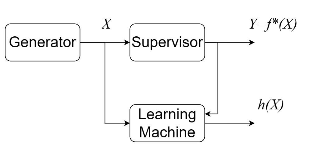
In the framework of statistical learning, we assume that there is a data generator and a supervisor. The function of the data generator is to generate data \(X\) independently according to a fixed and unknown distribution \(\mu\). For each data \(X\), the supervisor will return a corresponding label \(Y\) according to a fixed but unknown function \(f^*(X)\).
For instance, in the task of face recognition, it is natural to assume that all human faces are generated from the same generator. For each face, there exists a corresponding label. Therefore, the supervisor can be seen as a mapping from faces to their true labels. The goal of face recognition is to predict the label of any face generated by the unknown generator (sampled from the unknown distribution \(\mu\)). If we have access to all faces drawn from \(\mu\) and the corresponding labels, then we could construct a map \(f^*(X)\) directly. Unfortunately, in practice we only have access to finite data pairs \(\{(X_1,Y_1), (X_2,Y_2), \cdots \}\). The goal of face recognition can be restated as constructing an approximate function of supervisor \(f^*(\cdot)\) based on finite data pairs (training data).
Now let’s answer the first two questions at the beginning. The goal of learning is to approximate the unknown function \(Y=f^*(X)\) for each \(X\). If we have access to infinity data independently drawn from \(\mu\) and the corresponding labels, then we could construct a map to approximate \(f^*(X)\) directly. Unfortunately, in practice we only have access to finite data pairs \(\{(X_1,Y_1), (X_2,Y_2), \cdots \}\). Thus, the input of learning is finite data pairs. Without loss generality, we set the number of data pairs to \(n\), then the dataset is \(S = \{(X_1,Y_1), (X_2,Y_2), \cdots (X_n,Y_n) \}.\) Intuitively speaking, the \textbf{generalization gap originates from this finite sample process}, which will be shown in the next subsection. Suppose we have a hypothesis/function space \(\mathcal{H}\) that may not contain \(f^*(x)\), the goal of learning is to find an optimal solution \(h \in \mathcal{H}\) with respect to \textbf{generalization error} \(R(h).\) That is, \(R(h)=\int l(h(X), Y) d \mu(X, Y) = \mathbb{E}_{(X,Y)}[l(h(X), Y)].\) In the following, we also use \(\mathbb{E} [l(h(X), Y)]\) to represent the population risk.
Generalization Error
Unfortunately, the underlying distribution \(\mu\) is unknown to us in practice. What we have access to is the dataset \(S\) which contains finite pairs of data \((X_i, Y_i)\). Here we define empirical risk as \(\hat{R}(h)=\frac{1}{n}\sum_{i=1}^n l(h(X_i), Y_i) .\) Generalization gap is defined as the distance between generalization error and empirical risk for any given hypothesis \(h\):
\[\text{gen}(h,S)=R(h) - \hat{R}(h).\]By the property of expectation of independent variables, it can be shown that the expectation of empirical risk is equal to the generalization error:
\(\mathbb{E}[\hat{R}(h)]=\mathbb{E}[\frac{1}{n}\sum_{i=1}^n l(h(X_i), Y_i)]=\frac{1}{n}\sum_{i=1}^n \mathbb{E}[l(h(X_i), Y_i)]\) \(=\frac{1}{n}\sum_{i=1}^n l(h(X), Y)=\frac{1}{n}\sum_{i=1}^n \mathbb{E}[R(h)]=R(h).\)
Based on the relationship between generalization error and empirical risk, it is natural to convert the Generalization Error Minimization problem to the Empirical Risk Minimization problem. Here we expect that the Minimizer of Empirical Risk also has good performance with respect to generalization error. But this is not always true, and this will definitely lead to an error term in the statistical framework. Actually, this process is the origin of the generalization gap. On the other hand, it can be seen that the larger the dataset is, the smaller the generalization gap is. Give a hypothesis \(h \in \mathcal{H}\), the performance of \(h\)can be measured by excess risk \(\text{Excess Risk}= R(h)-R(f^*).\)
Notice that we have a condition \(h\in \mathcal{H}\) and we do not require \(f^*\) to be a member of\(\mathcal{H}\). We denote the population risk minimizer \(h^*\) associated with \(R(h)\) by
\[h^* = \text{argmin}_{h \in \mathcal{H}} R(h).\]Then the excess risk \(R(h)-R(f^*)\) can be decomposed as \(R(h)-R(f^*)=R(h)- R(h^*) + R(h^*) - R(f^*),\)
where \(R(h^*) - R(f^*)\) is the approximation error, \(R(h)- R(h^*)\) is the estimation error.
Approximation error
The approximation error is determined by the distance between hypothesis space \(\mathcal{H}\) and the actual optimal function \(f^*\). The commonly used machine learning models contain linear models, kernel models, and neural network models. The emphasis of this chapter is the neural network model, therefore it is necessary to give the approximation ability of neural networks.
Theorem 2.1 (Universal approximation theorem in [1]) A continuous function defined on a bounded domain can be approximated by a sufficiently large shallow (two-layer) neural network.
Theorem 2.2 (Universal approximation theorem for ReLU function, Theorem 1 in [8]) For any Bochner–Lebesgue p-integrable function \({\displaystyle f:\mathbb{R}^{n}\rightarrow \mathbb{R}^{m}}\) and \({\displaystyle \epsilon >0}\), there exists a fully-connected ReLU network \({\displaystyle F}\) of width exactly \({\displaystyle d_{m}=\max(n+1,m)}\), satisfying
\[\int\|f(x)-F(x)\|^{p} \mathrm{~d} x<\epsilon\]Universal approximation theorems indicate that the approximation error of neural network models can be ignored. In other words, the hypothesis space of the neural network covers any integrable function with given error tolerance \(\epsilon\). In the following, we will focus on the estimation error.
Uniform Learning Framework
Uniform Convergence for Empirical Risk Minimization
Let \(\hat{h}_S\) be the minimizer of empirical risk \(\hat{R}(h)\), \(\hat{h}_S = \text{argmin}_{h \in \mathcal{H}}\hat{R}(h)=\text{argmin}_{h \in \mathbb{H}}\frac{1}{n}\sum_{i=1}^n l(h(X_i), Y_i).\) In the Empirical Risk Minimization setting, the estimation error is determined by the distance between \(\hat{h}_S\) and the population risk minimizer \(h^*\).
It can be seen that estimation error can be bounded by generalization gap in uniformly learning framework:
Let \(\hat{h}_S\) be the minimizer of empirical risk \(\hat{R}(h)\), \(\hat{h}_S = \text{argmin}_{h \in \mathcal{H}}\hat{R}(h)=\text{argmin}_{h \in \mathbb{H}}\frac{1}{n}\sum_{i=1}^n l(h(X_i), Y_i).\) In the Empirical Risk Minimization setting, the estimation error is determined by the distance between \(\hat{h}_S\) and the population risk minimizer \(h^*\).
It can be seen that estimation error can be bounded by generalization gap in uniformly learning framework: \(R(\hat{h}_S) - R({h}^*) = R(\hat{h}_S) - \hat{R}(\hat{h}_S) + \hat{R}(\hat{h}_S) + \hat{R}({h}^*) - \hat{R}({h}^*) - R({h}^*) \\ \leq R(\hat{h}_S) - \hat{R}(\hat{h}_S) + \hat{R}({h}^*) - R({h}^*) \\ \leq \max_{h \in \mathcal{H}}\{ R({h}) - \hat{R}({h}) \} + \max_{h \in \mathcal{H}}\{ \hat{R}({h}) - R({h})\} \\ \leq 2 \max_{h \in \mathcal{H}} \{ |R({h}) - \hat{R}({h})| \}\)
The first inequality follows from the fact that \(\hat{R}(\hat{h}_S) - \hat{R}({h}^*) \leq 0 (\hat{h}_S = \text{argmin}_{h \in \mathcal{H}}\hat{R}(h)).\)
The decomposition technique used in the uniform learning framework is classical. The idea behind uniformly learning is to use the supremum over the hypothesis space \(\mathcal{H}\) to replace \(h^*\) and \(\hat{h}_{S}.\) Though there exists an optimal \(h^*\) and a hypothesis \(\hat{h}_{S}\) in \(\mathcal{H}.\) We do not know other properties of \(\hat{h}\) and \(h^*.\) Therefore, the uniform learning framework is a straightforward method to get the upper bound of estimation error. However, the use of supremum also leads to the main drawback of this framework.
Optimization Aspects
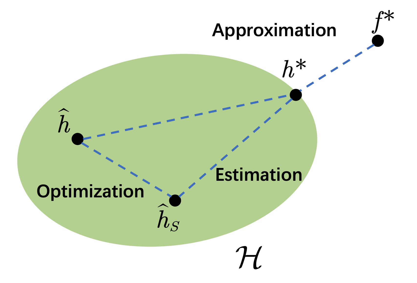
In the ERM setting, we focus on the empirical risk minimizer \(\hat{h}_S.\) However, the general hypothesis of interest is the output of the optimized algorithm (SGD), which may not be exact \(\hat{h}_S.\) Let \(\hat{h}\) be the approximated minimizer of empirical risk, then the new error \(R(\hat{h})- R(h^*)\) can be decomposed as \(R(\hat{h})- R({h}^*) = R(\hat{h}) - R(\hat{h}_S) + R(\hat{h}_S) - R({h}^*),\) where \({R}(\hat{h}) - {R}(\hat{h}_S)\) is the optimization error and \(R(\hat{h}_S) - R({h}^*)\) is the estimation error.
Based on this uniform learning framework, the estimation error \(R(\hat{h})-R(h^*)\) can be decomposed as \(R(\hat{h})-R(h^*) \leq R(\hat{h})- R(\hat{h}_S) + 2 \max_{h \in \mathcal{H}} \{ |R({h}) - \hat{R}({h})| \}\) where the first term is the optimization error and the last two terms are statistical errors. Looking at the right side of this inequality, we can get the key insight into the tradeoff between optimization error and statistic error, which can be described as follows. It is enough to run the optimization process until the order of optimization error is the same as the statistical error. The statistical error comes from the finite sample process and depends on the size of the dataset. It is pointless to run optimization processes to get a smaller optimization error than the statistical error.
Bounds in expectation and in probability
For any given underlying distribution \(\mu\) and hypothesis space \(\mathcal{H}\), \(R({h}^*)\) is determined. We recall that \(\hat{h}_S\) is induced by dataset \(S\). Therefore, \(R(\hat{h}_S)\) is random and its randomness comes from the sampling process of \(S\). Let’s take excess risk \(R(\hat{h}_S) - R({h}^*)\) as a random variable. There are two ways to bound excess risk, one is in expectation, and the other is in probability.
Bounds in expectation:
\[\mathbb{E}_{S}[R(\hat{h}_S) - R({h}^*)]=\mathbb{E}_{S}[R(\hat{h}_S)] - R({h}^*) \leq \text{Expectation}\]The upper bound in expectation reflects the average value of excess risk. The expectation is operated on dataset \(S\). When we use a deterministic learning algorithm, the uncertainty of \(\hat{h}^*\) only depends on \(S\). The bounds in expectation form reflect the average performance of the model optimized based on the randomly sampled datasets. The theoretical bounds in probability form, which we define in the following, reflect the performance of a single sampling on datasets.
Bounds in probability: \(\mathbb{P}\{R(\hat{h}_S) - R({h}^*) \geq \epsilon \} \leq \text{UpperTail}(\epsilon),\) where \(\epsilon \geq 0\). Or equivalently, for any \(\delta \in [0,1]\) \(\mathbb{P}\{R(\hat{h}_S) - R({h}^*) \leq \text{UpperTail}^{-1}(\delta) \} \geq 1-\delta .\)
Probability tools: Concentration inequalities
Concentration phenomenon
The Law of Large Number states that as a sample size grows, the average of sampled variables approaches to the mean value of the random variable. A similar concentration phenomenon can be seen for the function of sampled variables. That is,
Concentration phenomenon: If \(X_{1}, \ldots, X_{n}\) are independent random variables, then \(f\left(X_{1}, \ldots, X_{n}\right)\) is “close” to its mean \(\mathbb{E}\left[f\left(X_{1}, \ldots, X_{n}\right)\right]\) provided that \(X_{1}, \ldots, X_{n} \rightarrow f\left(X_{1}, \ldots, X_{n}\right)\) is not too “sensitive” to any of the coordinates \(X_{i}.\)
In the special case where \(X_{1}, \ldots, X_{n}\) are independent identically distributed (i.i.d.) and \(f(X_1, \cdots, X_n) = \frac{1}{n}\sum_{i=1}^{n}X_i,\) concentration phenomenon is a property of a large number of variables. Next, we explain this in more detail. If \(X_{1}, \ldots, X_{n}\) are i.i.d. random variables with mean \(\mu\) :
\[\left\{\mathbb{E}\left[\frac{1}{n} \sum_{i=1}^{n} X_{i}-\mu\right]^p\right\}^{1/p}\leq \frac{c_p}{\sqrt{n}}.\]Let \(p=2\), this inequality indicates that the variance of random \(\frac{1}{n}\sum_{i=1}^{n}X_i\) can be bounded by \(\frac{c_p^2}{n}\). That is, the variance convergence with a rate of order \(\mathcal{O}\left(\frac{1}{n}\right).\) As the sample size \(n\) increases, the variance of the sample mean approaches \(0\).
Hoeffding’s inequality
To get the upper bound of generalization error in probability form, we need to capture the concentration phenomenon in probability: \(\mathbb{P}\left(f\left(Z_{1}, \ldots, Z_{n}\right)-\mathbb{E} f\left(Z_{1}, \ldots, Z_{n}\right) \geq \varepsilon\right) \leq \operatorname{UpperTail}_{f}(\varepsilon), \\ \mathbb{P}\left(f\left(Z_{1}, \ldots, Z_{n}\right)-\mathbb{E} f\left(Z_{1}, \ldots, Z_{n}\right)<\operatorname{UpperTail}_{f}^{-1}(\delta)\right) \geq 1-\delta.\)
We provide the following useful concentration inequalities without proof.
Theorem 4.1 (Hoeffding’s inequality) Suppose that the variables \(X_i, i=1, \ldots, n\), are independent, and \(X_i\) has mean \(\mu_i\) and \(X_i \in [a,b] \). Then for all \(\epsilon \geq 0\), we have \(\mathbb{P}\left[\frac{1}{n}\sum_{i=1}^n\left(X_i-\mu_i\right) \geq \epsilon\right] \leq \exp \left\{-\frac{2n \epsilon^2}{(b-a)^2 }\right\}; \\ \mathbb{P}\left[\frac{1}{n}\sum_{i=1}^n\left(X_i-\mu_i\right) \leq -\epsilon\right] \leq \exp \left\{-\frac{2n \epsilon^2}{(b-a)^2 }\right\}.\)
Consequently, \(\mathbb{P}\left[ \left| \frac{1}{n}\sum_{i=1}^n\left(X_i-\mu_i\right) \right| \leq -\epsilon\right] \leq 2 \exp \left\{-\frac{2n \epsilon^2}{(b-a)^2 }\right\}.\) Hoeffding’s inequality captures the concentration phenomenon for the summation of finite independent random variables. By setting \(X_i \leftarrow \ell(h(X_i), Y_i), \) we are able to analyze the concentration phenomenon of empirical risk \(\hat{R}(h)\). The upper bounds for the generalization gap directly follow functional Hoeffding’s inequality:
Theorem 4.2 (Generalization Gap) If for any distribution \(P\) and each \(h\in \mathcal{H}\) we have \(\ell(h(X),Y) \in [0,1]\) , it follows that for any \(\epsilon \geq 0\): \(\mathbb{P} [\hat{R}(h)-R(h) \geq \epsilon] \leq e^{-2 n \epsilon^2}; \\ \mathbb{P} [\hat{R}(h)-R(h) \leq-\epsilon] \leq e^{-2 n \epsilon^2}.\)
Generalization error based on Complexity Measure
Generalization Bounds for Finite Hypothesis Sets
We first prove the generalization error bound for finite hypothesis space. Note that finite hypothesis space is strict since most Hypothesis Spaces contain infinite hypotheses. However, in computer science, any infinite hypothesis set can be converted into a finite version through quantification.
Theorem 5.1 (Generalization error for Finite Hypothesis Space) If for any distribution \(\mu\) and each \(h\in \mathcal{H}\) we have \(\ell(h(X),Y) \in [0,1]\) , with probability at least \(1-\delta\) we have \(\max_{h \in \mathcal{H}} \{ |R({h}) - \hat{R}({h})| \} \leq \sqrt{\frac{\log |\mathcal{H}| + \log(2/\delta)}{2n}}\)
\[\mathbb{P} \left[\max _{h \in \mathcal{H}}\left|R(h)-\widehat{R}_S(h)\right|>\epsilon\right] \\ =\mathbb{P}\left[\left|R\left(h_1\right)-\widehat{R}_S\left(h_1\right)\right|>\epsilon \vee \ldots \vee\left|R\left(h_{|\mathcal{H}|}\right)-\widehat{R}_S\left(h_{|\mathcal{H}|}\right)\right|>\epsilon\right] \\ \leq \sum_{h \in \mathcal{H}} \mathbb{P}\left[\left|R(h)-\widehat{R}_S(h)\right|>\epsilon\right] \\ \leq 2|\mathcal{H}| \exp (-2 n \epsilon^2).\]where the first inequality is due to Union bound and the second inequality is due to Hoeffding’s inequality.
By Setting \(\delta = 2 | \mathcal{H} | \exp{(-2n\epsilon^2)}\) and solving the inverse function, we get \(\epsilon = \sqrt{\frac{1}{2n} \log (\frac{2 |\mathcal{H}|}{\delta})} = \sqrt{\frac{\log |\mathcal{H}| + \log(2/\delta)}{2n}}\)
Generalization Bounds for Neural Networks
Rademacher Complexity is another method that reflects the “size” of hypothesis space \(\mathcal{H}\). Intuitively, Rademacher Complexity measures how well a hypothesis class can fit random noise. A higher Rademacher complexity implies that the hypothesis space \(\mathcal{H}\) is able to fit random labels well. In the following, we provide generalization error bounds of neural networks derived based on Rademacher Complexity.
Theorem 5.2 (Generalization error of Neural Networks, Proposition 3.6 in [9]) Consider a neural network hypothesis \(\mathcal{H}\) with \(L\) layers. Let \(W_i\) be the weight of \(i\)-th layer and \(\sigma\) be the active function. That is, \(\mathcal{H}:=\left\{X \mapsto \sigma_L\left(W_L \sigma_{L_1}\left(\cdots \sigma_1\left(W_1 X\right) \cdots\right)\right):\left\|W_i\right\|_{\mathrm{F}} \leq B\right\}.\) where \(\left\|W_i\right\|_{\mathrm{F}}\) the Frobenius Norm of weight \(W_i\). Let \(\| X \|\) be the norm of input vector. If for any distribution \(\mu\) and each \(h\in \mathcal{H}\) we have \(\ell(h(X),Y) \in [0,1]\) and \(\| X \| \leq 1.\) Then, with probability at least \(1-\delta\) \(\sup _{h \in \mathcal{H}} \{ R(h)-\hat{R}(h) \} \leq \frac{2B^L}{\sqrt{n}} (1+\sqrt{2 L \ln (2)}) +3\sqrt{\frac{\ln (2 / \delta)}{2 n}}.\)
Theorem 5.2 demonstrates that to achieve good generalization guarantees one needs to use a training sample size \(n\) that exceeds the “complexity” of the learning model \(B^L.\) In practice, the total number of neural networks \(L\) is large. Thus, it is too restrictive to require training sample size to exceed \(B^L.\) On the other hand, it is clear that \(\sup _{h \in \mathcal{H}} \{ R(h)-\hat{R}(h) \} \leq 1\) when the loss function satisfies \(\ell(h(X),Y) \in [0,1].\) However, the right side of inequality (equation above) would be larger than \(1\) when \(n\) is small, in which case the Theorem 5.2 is meaningless. Investigating meaningful generalization error bounds for neural networks is an active topic. In the next Section, we introduce the meaningful bounds derived based on information-theoretic tools.
An Information-Theoretic View for Deep Learning
As we point out in the previous section, classical methods such as Rademacher complexity and Stability fail to give non-vacuous generalization bounds for neural networks. Intuitively, both algorithm \(\mathcal{A}\) and data distribution \(\mu\) affect the generalization performance of the learned model. However, the complexity-based approaches only capture the influence of data distribution \(\mu\). The stability-based approaches only reflect the influence of the algorithm \(\mathcal{A}\). By contrast, generalization bounds derived based on information theory capture the influence of both factors (algorithm \(\mathcal{A}\) and data distribution \(\mu\)). Moreover, it will be shown that information-theoretic tools have the potential to provide more insights into understanding deep learning. In this section, we focus on the Information-Theoretic results for deep learning, which contains not only the generalization error bounds but also different perspectives in understanding the mystery of deep learning.
Basics of information theory
Information theory makes fundamental contributions in many fields, including wireless communication, computer science, and statistical physics. The basic concepts of information theory were proposed by Claude Shannon in the 1940s. In recent years, information theory has been applied in the analysis of deep learning from different aspects. To understand the basic concepts of information theory, we begin with a communication model described as follows.
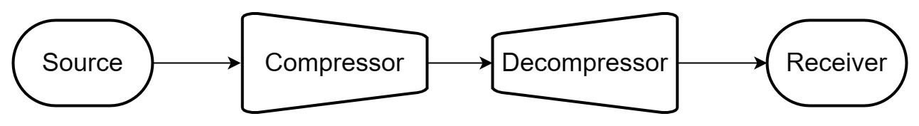
In wireless communication systems, the main challenge is how to improve the data transmission speed. Two ways can be used to tackle such a challenge. One is to compress the source data, the other is to improve the transmission throughput. Information theory answers two fundamental questions in the analysis of data compression and transmission: what is the limitation of compression and what is the limitation of transmission throughput? The answer to the first question is Entropy. Readers interested in the second question can refer to “The element of information theory (Book)”.
Entropy, Relative Entropy, and Mutual Information
Consider \(X \in \mathcal{X}\) as a finite random variable with distribution \(P\) and let \(p\) denote the corresponding probability mass function. That is \(P(X=x) = p(x).\) The \textbf{entropy} of \(X\) is defined as \(H(X):=-\sum_x p(x) \log p(x).\)
For random variables with probability mass function \(p\), Entropy is defined as the weighted summation of \(\log \frac{1}{p(x)}\). In other words, the larger the probability \(P(X=x)\), the smaller this term \(\log \frac{1}{p(x)}\) will be. One natural question is, why Shannon chose this term for the definition of entropy? To answer this question, we need to recall the communication systems. The goal of defining the concept of Entropy is to analyze the limitation of data compression. To improve the compression rate, the natural idea is to use short sequences to represent the random values with high probability and use long sequences to represent the low probability random values. Then the average length used to represent the random variable \(X\) will be as short as possible.
Let \(q(x)\) be another probability mass function defined on \(\mathcal{X}\), then the difference between \(p(x)\) and \(q(x)\) can be measured by \textbf{relative entropy (Kullback Leibler Divergence)}: \(D[p \| q]=\sum_{x \in \mathcal{X}} p(x) \log \left(\frac{p(x)}{q(x)}\right).\) It can be proved that KL divergence is positive (See proof in [13]).
Consider \(Y \in \mathcal{Y}\) as random variables with probability mass function \(p(y)\) and let \(p(x,y)\) denote the joint distribution function of \(X\) and \(Y\). The Mutual Information between \(X\) and \(Y\) is defined as: \(I(X ; Y)=\sum_{x \in \mathcal{X}, y \in \mathcal{Y}} p(x, y) \log \frac{p(x, y)}{p(x) p(y)}.\) Intuitively, mutual information is a measurement of the dependence between \(X\) and \(Y\). The more dependence between \(X\) and \(Y\), the larger the mutual information will be. Mutual Information can be seen as the KL divergence of \(p(x,y)\) and \(p(x)p(y)\). Thus, mutual information is positive.
Generalization Error via Mutual Information
Theorem 6.1 (Theorem 1 in [15]) If \(\forall w \in \mathcal{W}, \forall Z\in \mathcal{Z}, |\ell(Z, w)| \leq M\), then for every algorithm output \(\mathcal{A}\), the generalization error of is bounded by \(|\mathbb{E}[\operatorname{gen}(S, W)]| \leq \sqrt{\frac{ M^{2}}{2n} I(S ; W)}.\) Where \(W\) represents the parameters of the machine learning model, \(S\) is the dataset we used to train the model. Theoretical results based on information theory tell us that the generalization error of Neural Networks is bounded by the mutual information \(I(W,S)\). Mutual information is a measure of dependence between two random variables. If the model parameter \(W\) is completely determined by dataset \(S\), then the mutual information will be large. In that case, we can say that the model just “remembers” the dataset rather than “learning” from it. Intuitively speaking, based on this learning bound, we could say that a good model should not only remember the dataset.
Understanding Deep Learning via Rate-Distortion Theory
It has been shown that neural networks can be compressed/pruned without damaging generalization performance. In this subsection, we provide explicit theoretical generalization bounds reflecting the compressibility of neural networks. Rate distortion theory is developed in the field of communication. It provides theoretical guarantees on the minimum Entropy used to present random variable \(X\) when compression and decompression are allowed to lose some information of \(X\). Since neural networks can be compressed without loss of performance, it is natural to relate rate-distortion theory and the generalization error of neural networks.
In the following, we present the generalization bounds derived based on the rate-distortion theory, which reflects the compressibility of neural networks.
Theorem 6.2 (Theorem 4 in [10]) If \(\forall w \in \mathcal{W}, \forall Z\in \mathcal{Z}, |\ell(Z, w)| \leq M\), then for every algorithm \(\mathcal{A}\) and every \(\epsilon \in \mathbb{R}\), \(|\mathbb{E}[\operatorname{gen}(S, W)]| \leq \sqrt{\frac{2 M^2 I\left(\epsilon, P_{S, W}\right)}{n}}+\epsilon,\) where \(I\left(\epsilon, P_{S,W}\right)=\min I(S ; \hat{W})\) such that \(|\mathbb{E}[\operatorname{gen}(S, W)-\operatorname{gen}(S, \hat{W})]| \leq \epsilon.\)
Compared to classical generalization bound derived based on information theory, this bound involves mutual information \(\min I(S ; \hat{W})\) instead of \(I(W;S)\). Here \(\hat{W}\) needs to satisfy \(\|\mathbb{E}[\operatorname{gen}(S, W)-\operatorname{gen}(S, \hat{W})]\|\leq \epsilon\). Note that \(\min I(S ; \hat{W})\) may be much less than \(I(W;S)\). Let’s explain the insights behind this theorem. \(\hat{W}\) can be seen as the compressed version of original\(W\). Thus, for any compressed \(\hat{W}\) satisfying \(\|\mathbb{E}[\operatorname{gen}(S, W)-\operatorname{gen}(S, \hat{W})]\| \leq \epsilon\), the generalization error is bounded by mutual information \(I(S; \hat{W})\). In other words, if we can find some compressed models \(\hat{W}\) whose performance is similar to the original model \(W\), then it can be guaranteed that the generalization error of the original model is bounded by \(\min I(S ; \hat{W})\) (minimum dependence between \(S\) and compressed model \(\hat{W}\) ).
Out of Distribution generalization via Information theory
In practice, the underlying distribution \(\mu\) of training data may be different from the distribution of test data. This mismatch phenomenon appears in many fields, including healthcare, drug discovery, and computational mechanics. We denote the test distribution by \(\mu^{\prime}\). The generalization error associated with \(\mu^{\prime}\) is defined as \(R_{\mu^{\prime}}(W)=\mathbb{E}_{Z\sim \mu^{\prime}}[\ell(Z, W)].\)
The generalization error bound under distribution mismatch can be derived as follows:
Theorem 6.3 (Corollary 2 in [14]) If \(\forall w \in \mathcal{W}, \forall Z\in \mathcal{Z}, |\ell(Z, w)| \leq M\), then for every algorithm \({A}\), it follows that \(\mathbb{E}\left[R_{\mu^{\prime}}(W)-\hat{R}(W, S)\right] \leq \sqrt{2 M^2\left(\frac{I(W ; S)}{n}+D\left(\mu \| \mu^{\prime}\right)\right)},\)
Compared to the classical setting, generalization bound under distribution mismatch has an extra Relative Entropy term \(D\left(\mu \| \mu^{\prime}\right)\). Intuitively, it can be guaranteed that the generalization associated with mismatch distribution will be small if the distance between \(\mu^{\prime}\) and \(\mu\) is small. In other words, one can not expect to get good generalization performance if the distance between \(\mu^{\prime}\) and \(\mu\) is large. This is consistent with the No free lunch theorem.
Information Flow in Deep Learning
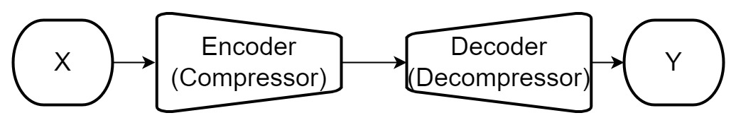
Learning is the process of finding a proper mapping/function from input \(X\) to \(Y\). In general, the dimension of input \(X\) is very high (e.g., images). The basic idea of representation learning is that there exists a (low-dimension) representation \(T\) of input data \(X\), which can be used to make further predictions/decisions. It is crucial and natural to ask the first question: which kind of representation is good? Inspired by signal processing and neural science, many efforts have been made to answer this question. From the perspective of neural science, a potential answer is that good representation has low-dimension structures. Finding low-dimension structures is the key to the efficiency of the brain. From the perspective of signal processing/information theory, low-dimension structures correspond to low Entropy.
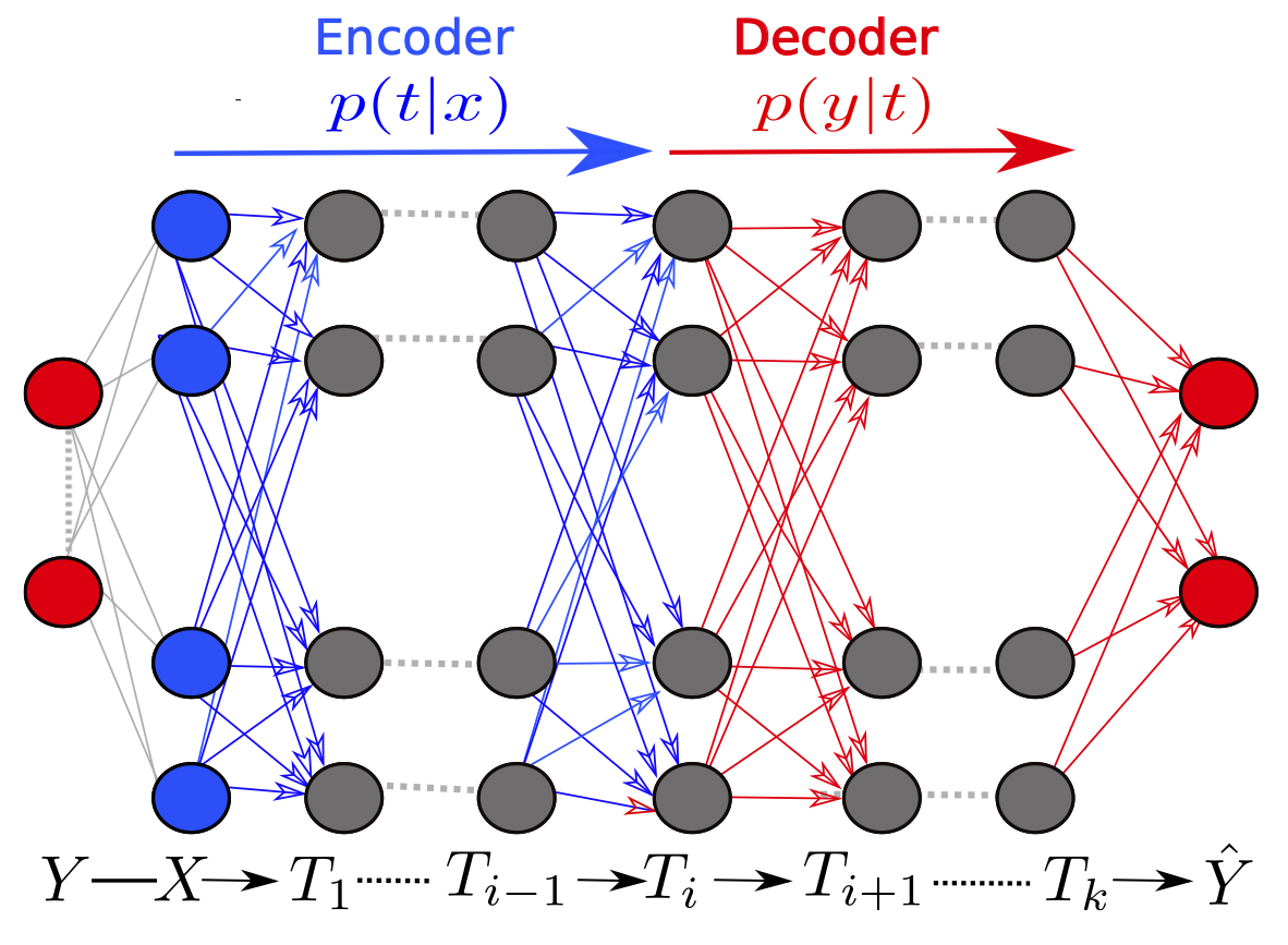
Intuitively, finding good representation can be seen as compression, and predicting based on the representation can be seen as decompression. We provide an explanation of neural network training based on this framework in the following. Suppose the input is \(X\) and the target is \(Y\), a good presentation \(T\) should satisfy two conditions. One is that \(T\) should be compressed as much as possible, which means that \(I(X;T)\) should be as. The other is that \(T\) should capture information about \(Y\) that is available in \(X\) as much as possible. That is, \(I(T;Y)\) should be large. This tradeoff can be expressed as \(\min \{I(X ; T)-\beta I(T ; Y)\},\) where \(\beta\) is a parameter used to balance these two terms.
Let \(T_i\) be the compressed representation of \(X\) in \(i\)-layer and \(\hat{Y}\) be the output of the neural network. Based on the previous formulation, we could visualize the information flow during training.
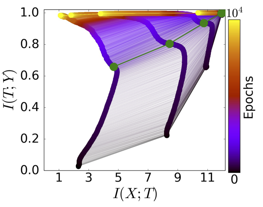
As shown in this figure, the training process can be divided into two phases.
- \(I(X;T_i)\) increases in the first phase and decreases in the second phase, which means that memorization happens in the first phase and compression happens in the second phase.
- \(I(Y;T_i)\) increases in both phases, which means that the generalization error decreases monotonously along the training process.
- The output of deeper layer \(T_i\) corresponds to smaller \(I(Y;T_i)\) , which is consistent with the theoretical analysis based on information theory.
Theorem 6.4 (Information Flow across Different Layers) Let \(T_j\) be the output of \(j\)-th layer and denote the output of the last hidden layer by \(T_k\), then we have \(I(Y ; X) \geq I\left(Y ; T_j\right) \geq I\left(Y ; T_k\right) \geq I(Y ; \hat{Y}),\) where \(X\) represent the input feature, \(Y\) represent the input label and \(\hat{Y}\) is the output of neural network.
If \(X,Y\)are random variables, \(Z=f(Y)\), where \(f(\cdot)\) is a determined function, then \(I(X;Y) \geq I(X;Z).\) This property shows that the information contained in \(Y\) of \(X\) cannot be increased by processing \(Y\). For more details, see the data processing inequality part in [2].
Network Compression
Since the limitation of computational resources, network compression is a widely used technique in practice. The goal of network compression is to find a small network that has similar or even better performance than the original large network. The most interesting phenomenon of network compression is Lottery Ticket Hypothesis. In this subsection, we first describe this phenomenon. Then we provide the notable theoretical analysis results of the Lottery Ticket Hypothesis.
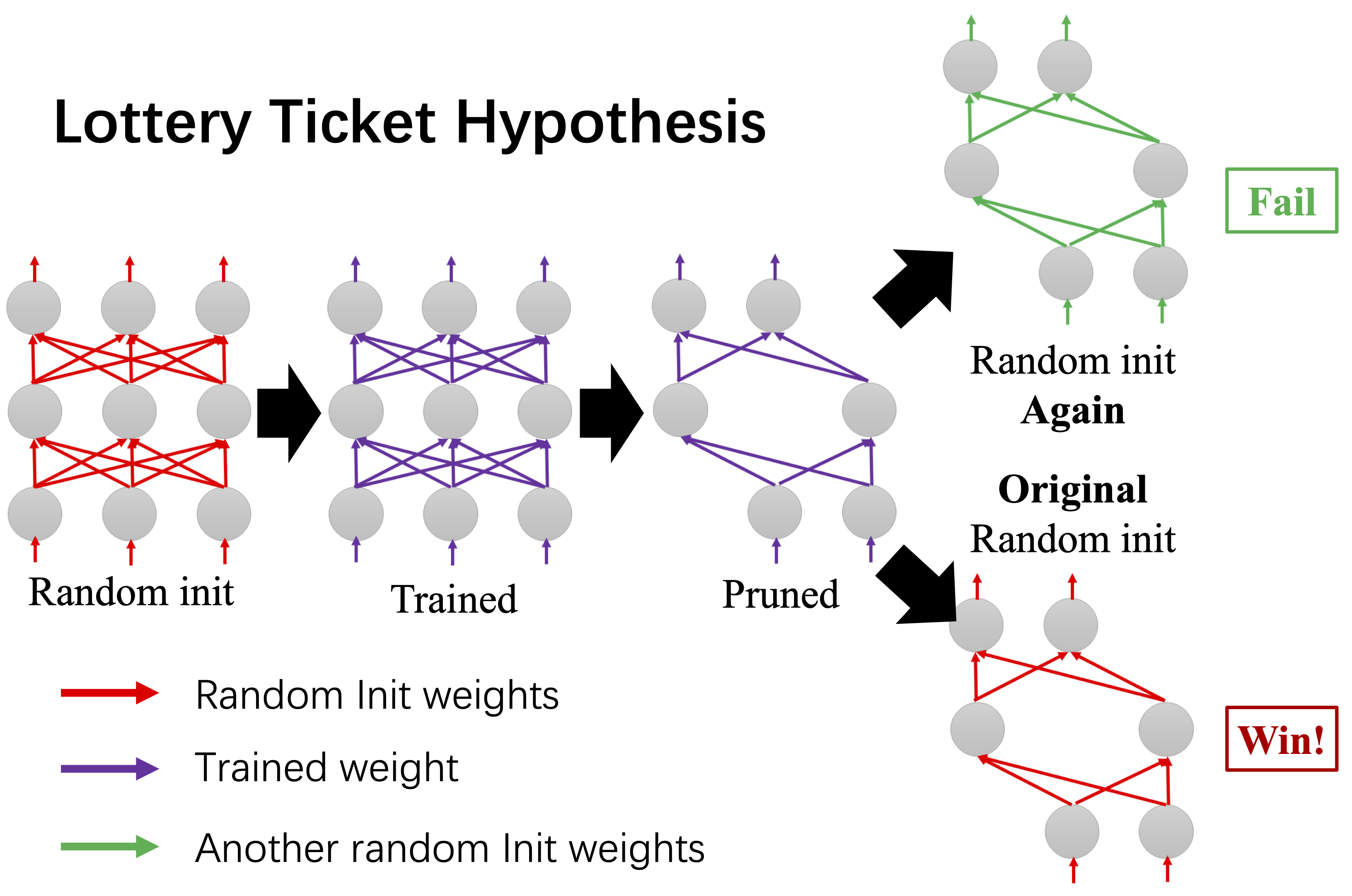
As shown in the figure, the trained model can be pruned by removing the neurons that are not significant. Then the pruned model can be retrained based on two types of initialization methods. One is random initialization. The other is using the original random initialization. It can be shown that the performance of the second method matches the original model. The first initialization method fails to get good performance. The winning subnetworks (tickets) are called Lottery Ticket Hypothesis. The existence of the Lottery Ticket Hypothesis is proved by systematic empirical analysis in [17]. we theoretically explain why the Lottery Ticket Hypothesis wins.
Why Lottery Ticket Hypothesis Wins?
Take one-hidden layer as an example, [16] provides the following results
Theorem 6.5 (Local Convexity near optimal, Theorem 1 in [16]) Pruning enlarges the convex region of the empirical loss landscape where the generalization error is small.
Theorem 6.5 indicates that training on pruned sub-network may lead to easier estimation of an optimal model. It is well known that the loss landscape of neural networks is non-convex and has local minima. Therefore, it is easier to approach the optimal model if the convex region is enlarged.
Theorem 6.6 (Convergence of pruned model, Theorem 2 in [16]) 1) Pruned sub-network needs a smaller sample size to achieve successful convergence. 2) Pruned sub-network convergences faster with the same sample size.
Theorem 6.6 indicates that the pruned sub-network convergences faster than the original network. Theorem 1 provides guarantees on the generalization performance of pruned sub-network. Theorem 6.6 provides guarantees on the optimization performance of pruned sub-network. These two theorems provide theoretical guarantees on the benefit of pruning/compression. Though the theoretical analysis of these results is developed for the one-hidden layer neural network, further experimental results are provided for the multi-layer neural network to justify the universality of the theory.
Future Reading
The goal of this chapter is to provide theoretical insights into why and how deep learning can generalize well. Many topics are not covered and many more are not covered in much depth. For a deeper understanding of the classical machine learning theory, we recommend the excellent textbooks of [11]and [7]. See also the nice notes from [6], [3] as well as from [9]. For a deeper understanding of the deep learning theory, we recommend the systematic survey by [4].
Appendix
Lemma 8.1 (Markov’s Inequality) For any non-negative random variable \(X\) we have, for any \(\varepsilon \geq 0\), we have \(\mathbb{P}(X \geq \varepsilon) \leq \frac{\mathbb{E} X}{\varepsilon}.\)
For a continuous non-negative random variable \(X\) with probability density \(p\),
\(\mathbb{E}(X) =\int_{0}^{\infty} Xp(X) d X=\int_{0}^{a} Xp(X) d X+\int_{a}^{\infty} Xp(X) d X\\ \geq \int_{a}^{\infty} Xp(X) d X\geq a \int_{a}^{\infty} p(X) d X=a \mathbb{P}(X \geq a)\) Thus, \(\mathbb{P}(x \geq a) \leq \frac{\mathbb{E}(X)}{a}\)
Lemma 8.2 (Chernoff bound) For any random variable \(X\) and any \(\lambda \geq 0, \varepsilon \in \mathbb{R}\) we have, \(\mathbb{P}(X \geq \varepsilon) \leq \frac{\mathbb{E} e^{\lambda X}}{e^{\lambda \varepsilon}}\) Exponentiate and apply Markov’s inequality: \(\mathbb{P}(X \geq \varepsilon)=\mathbb{P}\left(e^{\lambda X} \geq e^{\lambda \varepsilon}\right) \leq \frac{\mathbb{E} e^{\lambda X}}{e^{\lambda \varepsilon}}\)
References
[1] Andrew R Barron. Universal approximation bounds for superpositions of a sigmoidal function. IEEE Transactions on Information theory, 39(3):930–945, 1993.
[2] T. M. Cover and J. A. Thomas. Elements of information theory 2nd edition. 2006.
[3] Bruce Hajek and Maxim Raginsky. Ece 543: Statistical learning theory. University of Illinois lecture notes, 2019.
[4] Fengxiang He and Dacheng Tao. Recent advances in deep learning theory. arXiv preprint arXiv:2012.10931, 2020.
[5] Hung-Yi Lee. Lecture Notes for Machine Learning. https://github.com/virginiakm1988/ML2022-Spring/, 2022. [Online; accessed 14-February-2023].
[6] Tengyu Ma. Lecture Notes for Machine Learning Theory.https://web.stanford.edu/class/stats214/, 2022. [Online; accessed 1-February-2023].
[7] Mehryar Mohri, Afshin Rostamizadeh, and Ameet Talwalkar. Foundations of machine learning. MIT press,2018.
[8] Sejun Park, Chulhee Yun, Jaeho Lee, and Jinwoo Shin. Minimum width for universal approximation. In International Conference on Learning Representations, 2021. URL https://openreview.net/forum?id=O-XJwyoIF-k.
[9] Patrick Rebeschini. Algorithmic Foundations of Learning. https://www.stats.ox.ac.uk/~rebeschi/teaching/AFoL/22/index.html, 2022. [Online; accessed 1-February-2023].
[10] Milad Sefidgaran, Amin Gohari, Gael Richard, and Umut Simsekli. Rate-distortion theoretic generalization bounds for stochastic learning algorithms. In Conference on Learning Theory, pages 4416–4463. PMLR, 2022.
[11] Shai Shalev-Shwartz and Shai Ben-David. Understanding machine learning: From theory to algorithms. Cambridge university press, 2014.
[12] Ravid Shwartz-Ziv. Information flow in deep neural networks. arXiv preprint arXiv:2202.06749, 2022.
[13] Joram Soch, The Book of Statistical Proofs, Thomas J. Faulkenberry, Kenneth Petrykowski, and Carsten Allefeld. StatProofBook/StatProofBook.github.io: StatProofBook 2020, December 2020. URL https://doi.org/10.5281/zenodo.4305950.
[14] Xuetong Wu, Jonathan H Manton, Uwe Aickelin, and Jingge Zhu. Information-theoretic analysis for transfer learning. In 2020 IEEE International Symposium on Information Theory (ISIT), pages 2819–2824. IEEE, 2020.
[15] Aolin Xu and Maxim Raginsky. Information-theoretic analysis of generalization capability of learning algorithms. Advances in Neural Information Processing Systems, 30, 2017.
[16] Shuai Zhang, Meng Wang, Sijia Liu, Pin-Yu Chen, and Jinjun Xiong. Why lottery ticket wins? a theoretical perspective of sample complexity on sparse neural networks. Advances in Neural Information Processing Systems, 34:2707–2720, 2021.
[17] Jonathan Frankle and Michael Carbin. The lottery ticket hypothesis: Finding sparse, trainable neural networks. In International Conference on Learning Representations