Author(s): Yanze Wang is a Ph.D. student @ MIT Chem and Broad Institute. He joined MIT and Broad Institute in 2022. He is a developer @Deepmodeling community. He is interested in molecular simulation and how computational tools help optimize bio-macromolecules with a special interest in RNA simulation.
Before you start
- This tutorial assumes that you have already learned:
-
Basic physics and chemistry knowledge
-
Calculus
-
- If you want to deeply understand the principles and roles of molecular dynamics, you need to master the following:
-
Mechanics, theoretical mechanics (analytical mechanics)
-
Statistical Mechanics
-
Physical Chemistry
-
Numerical Methods / Computational Physics / Computational Methods
-
Further topics:
- Quantum Chemistry
- Biochemistry or Solid State Physics, depending on the specific application
-
What is Molecular Dynamics?
Molecular Dynamics (MD) studies how atomic coordinates evolve under given conditions. It relies on the framework of classical mechanics(also known as Newtonian mechanics) and simulates the motion of molecular systems numerically. For instance, you can imagine the motion of two rigid balls connected by a spring.
Experiments on a computer
MD is a computational method, a chemical experiment performed on computers. Let’s imagine a chemical experiment in the real world first. One may have to prepare experimental instruments and drugs, set instrument parameters, conduct experiments, wait for chemical reactions to proceed, obtain experimental results, and then analyze experimental results. MD is quite similar; we use a table to compare MD with the traditional chemical experiments:
| Chemical experiment | Molecular dynamics simulation |
|---|---|
| Prepare experimental instruments | Prepare computing hardware (CPU, GPU, etc.) Prepare calculation software (Gromacs, Lammps, etc.) |
| Prepare experimental drugs | Prepare a file describing the molecular structure as an initial conformation for the simulation process |
| Set instrument parameters | Set simulation parameters (simulation temperature, simulation time, etc.) Set force field parameters (parameters that can be analogous to spring coefficients) |
| Conduct chemical experiments | Run MD simulations |
| Get experimental results | Get the simulated trajectory |
| Analyze experimental results | Analysis of physico-chemical properties from trajectories obtained from simulations (calculation of statistics) |
Why do we run MD?
Molecular dynamics simulations can allow us to simulate chemical and physical processes on computers, obtain kinetic information at the microscopic scale, provide theoretical support for experiments and guide chemical experiments. Moreover, computational simulations can help reduce the cost of manually conducting experiments. MD can also be performed under special (usually severe) conditions (ultra-high pressure, ultra-high temperature, strong electric field, magnetic field, etc.)
However, its basis in classical mechanics means that MD can only be effective for physical processes at the molecular scale (e.g. $nm$). For simulations involving electronic structures MD doesn’t work.
-
Systems that can be simulated with classical molecular dynamics:
-
Protein systems (protein folding problems, etc.)
-
RNA systems
-
Atomic-scale material systems
-
Free energy calculation
-
Catalytic reactions that do not involve electron transfer
-
-
Problems that classical MD can not solve (or cannot be solved only by classical MD):
-
Magnetic and electrical properties of materials (requires quantum chemistry tools)
-
Calculate the energy of molecular conformation (requires quantum chemistry method, current software include Gaussian, Vasp)
-
Protease-catalyzed reactions involving electron transfer (requires QM/MM method)
-
Chemical reactions involving electron transfer (requires QM/MM method)
-
The inputs and outputs of MD
Inputs to molecular dynamics simulations are an initial conformation of molecules. They should contain the coordinates of the atoms, the information of chemical bonds among atoms (also called topology information), etc.
The outputs of molecular dynamics are molecular trajectories (trajectory refers to a continuous molecular motion in the coordinate space or Cartesian space) simulated from the initial conformations.
Starting with a simple example
Here we consider a simple example of a molecular dynamics simulation for a hydrogen molecule in vacuum. \(H - H\) (a single hydrogen molecule)
Basic knowledge
Let’s go over some basic knowledge before simulations:
- Molecules have an associated energy, which can be divided to potential energy (denoted by V) and kinetic energy (denoted by T). Potential energy is related to the coordinates of the atoms in molecules, while kinetic energy is related to the velocity (or momentum) of the atoms.
where \(q\) represents the vector coordinates of atoms and \(p\) represents the momentum of atoms.
- Force is the negative derivative of the energy over coordinates. Since kinetic energy has nothing to do with positions (coordinates), force is also equal to the negative derivative of potential energy over coordinates.
The construction of theoretical models - generating force fields
Why do we need force fields?
To simulate the motion of hydrogen molecules, we need to know the forces exerted on hydrogen atoms at different positions. These can be used to calculate changes of velocity and coordinates. This is equivalent to knowing the potential energy surface of the H2 molecule.
How do we get the potential energy surface? The most straightforward way is to calculate the energy by solving Schrödinger equations, and then calculate forces from derivatives. Then our simulation process becomes:
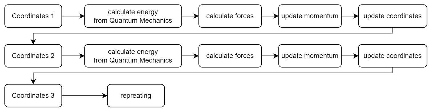
Every time we get a new position in the coordinate space, we need to solve a new set of Schrödinger equations. It is very time-consuming and laborious for complex systems. However, to calculate the motion of hydrogen atoms, we don’t need to know the exact information of the electrons in hydrogen atom, but only the position information of the nucleus. Thus we need the Born-Oppenheimer approximation.
The Born-Oppenheimer approximation is a quantum chemical approximation for electrons. Since nuclei are much heavier than electrons, they move much slower. We can assume that the motion of the nuclei is only affected by the mean-field of electrons.
Simply speaking, we only need to know the positions and forces about the hydrogen nucleus. The influence of electrons can be represented by some force field parameters under approximations. For example, we can approximate the hydrogen molecule as a spring model, and regard the interaction from electrons (or chemical bonds) as a spring. The force generated by the chemical bond is described by the spring coefficient. In this way, we transform the problem of solving Schrödinger equations to calculating the force of a spring:
\[F = k(x-x_0)\]where k represents the spring coefficient, and x0 represents the offset from the equilibrium position. As a result, calculations are greatly simplified. Here, the k (spring coefficient, or force constant) and x0 (equilibrium positions) are simplified force field parameters, also known as the force field.
Note that such simplification can significantly reduce the accuracy of MD simulations, so MD can only reflect the information near equilibrium states. But for macro statistics (e.g. chemical shift, protein contact), it is usually a sufficient description.
The actual force field parameters.
In real MD simulations, almost all inter-atomic and inter-molecular forces are approximated by an analytical expression of classical mechanics. These empirical parameters are obtained by fitting experimental data or data from quantum calculations}(for example, gradient descent optimization. Usually, the format of force fields looks like a combination of terms like:
\[U =\sum_{\text {bonds }} \frac{1}{2} k_{b}\left(r-r_{0}\right)^{2}+\sum_{\text {angles }} \frac{1}{2} k_{a}\left(\theta-\theta_{0}\right)^{2}+\sum_{\text {torsions }} \frac{V_{n}}{2}[1+\cos (n \phi-\delta)] +\] \[\sum_{\text {improper }} V_{i m p}+\sum_{\mathrm{LJ}} 4 \epsilon_{i j}\left(\frac{\sigma_{i j}^{12}}{r_{i j}^{12}}-\frac{\sigma_{i j}^{6}}{r_{i j}^{6}}\right)+\sum_{\text {elec }} \frac{q_{i} q_{j}}{r_{i j}}\]These interactions include:
-
Short-range interactions:
-
bonds
-
angles
-
torsion (dihedral angles)
-
-
Long-range interactions
-
Electrostatic interactions (Coulomb interactions, elec)
-
Van der Waals
-
Preparation for simulation
Now, we have modeled a hydrogen molecule. For simplicity, let the force constant of the hydrogen molecule be \(0.1 kJ/\mathring A^2\). Then let the equilibrium bond length be \(0.5\mathring A\), and the mass of the hydrogen atom is assumed to be (1) (just for demonstration).
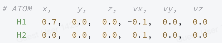
- To start the simulation, we also need the initial conditions (initial conformation and initial velocity). Also for simplicity, we assume that the coordinates of the two atoms are [0.7, 0, 0], [0, 0, 0] (Unit: angstrom), and the velocities are [-0.1, 0, 0], [0.1, 0 , 0] (Unit: angstrom/fs)
-
Next, let’s set the simulation parameters: since we calculate the differential equation numerically, we need to give the minimum simulation time interval, which is generally set to be 2 fs.(which is actually the grid size for time dimension in finite difference method).
-
Set the simulation to 5 steps, so the total simulation time is 10 fs.
-
Set the simulated temperature to 300K (this affects the velocity initialization and force field parameters, which should be set before velocity initialization).
Ready? Let’s simulate!
Simulation
(Please be aware that units are omitted for simplicity)
- Calculate the force on the hydrogen atoms from the initial positions:
- Calculate the accelerations:
- Update velocities:
-
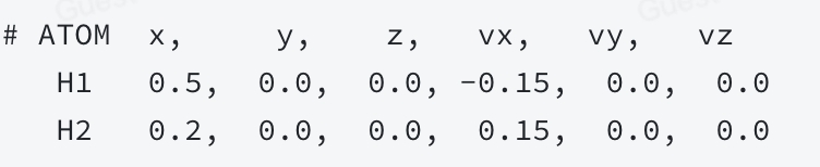
Update the coordinates and velocities through the calculation above to obtain new coordinates:
-
(Repeat) Calculate the new force
-
(Repeat) Calculate the new acceleration
Results
Finally, we will obtain positions of H atoms at different times, and these “continuous” motions compose the MD trajectory.
Through long-term MD simulations, we can calculate physical and chemical properties from the trajectories. (such as RMSD changes, conformation transitions, ensemble averaging of physical quantities, etc.)
Notes: Here, the equations from Newtonian mechanics are used for the purposes of demonstration. MD simulation is usually more complicated. Depending on the required ensemble, numerical evolution of partial differential equations will be carried out under specific Hamiltonian mechanics.
We will not introduce the concept of the ensemble in detail here. If you are interested in it, please read the related content about statistical mechanics.
An advanced example
In this part, we will use an example of a protein to illustrate how to conduct MD simulations in real-world research.
Building Model
Again, we use the BO approximation to construct models for proteins. These models include information on bond types, atom types, and force field parameters for various interactions. We usually need the following files:
-
topology (
topol.topfor example): Contains molecular bonding information, molecular type information, and atomic type information -
force field (
forcefield.itpfor example): contains chemical bond equilibrium positions, chemical bond force constants, non-bond force constants, etc. -
Commonly used force fields are as follows:
-
Amber
-
Charmm
-
Gromos
-
OPLS
-
-
So far there is no unified database or maintenance of methods for force fields, and each force field is maintained by each company or organization. Developing a force field is a difficult and nuanced process.
Solvent
Unlike systems in vacuum, proteins generally exist in solvents. We therefore need to account for and model the solvent. We can do this in two ways:
-
Explicit solvent model. It is often used in all-atom simulations, that is, directly introducing solvent molecules into the system. The force field parameters for solvent molecules are usually included in the force field file. Commonly used models for water are SCP, TIP3P, TIP4P, etc.
-
Advantages: Similar to the actual physical process, the results are more accurate. It can describe solvent-involved processes (e.g. protein-ligand binding). It can also explicitly describe solvent effects such as hydrogen bonding.
-
Disadvantages: high computational complexity. A system usually contains hundreds or thousands of solvent molecules.
-
-
Implicit solvent model. The effect of the solvent on the solute is described by a continuous electric field model. The Generalized Born model is an example of commonly used model.
-
Advantages: low computational complexity, no need to introduce additional solvent molecules.
-
Disadvantages: Imprecise, solvent-involved reactions cannot be described.
-
-
Periodic Boundary Conditions:
Due to limited computation resources it is impossible for us to simulate an infinitely large system, nor to simulate infinite steps. For a protein system, tens of thousands of atoms already require a lot of calculations (the required calculation time is measured in days), but this is still far less than Avogadro’s constant(1023).
However, simulating a small system will be seriously affected by the interface and cannot reflect the properties of the bulk phase.
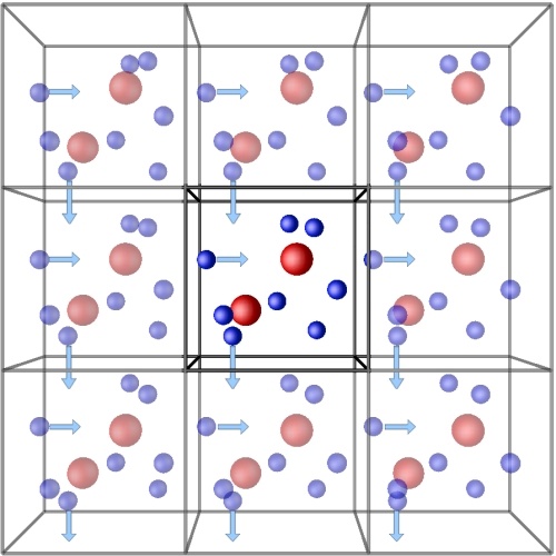
To solve this problem, we often use periodic boundary conditions. We confine the system of interest in a box and assume the properties of the actual system can be approximated by an virtual infinite system of repeating side-by-side lattices. If the molecule passes through the box boundary, it will re-enter the box from the opposite boundary, forming a periodic space.
-
Preparation for simulation
Next, you need to prepare the conformation files of the protein and water molecules. Typically, protein structure files are generated by PDBs, then converted into a format that can be read by molecular dynamics software.
We also need to prepare simulation parameter files, in which you need to set:
-
temperature
-
time interval and duration for simulations
-
the integrator/numerical algorithm, the ensemble for simulations
-
the temperature/pressure controller
-
the output-frequency and content of output files
-
-
Simulation Commonly used MD simulation software in current research are as follows:
-
Amber [1]
- Commercial software. There is a free version and a high-performance optimized commercial version. The code is closed source and highly engineered. It supports most MD functions and plays an important role in the simulation of protein systems. Amber is often used in simulations of biological systems.
-
Gromacs [2]
- Open-source MD simulation software. The latest release is the Gromacs 2022 release version. With efficient GPU optimization, there is a good developer community for Gromacs. This is mostly used for biological system simulation.
-
OpenMM [3]
- Molecular dynamics simulation software with Python interfaces. Modules are implemented by calling functions from the Python command line, which can directly involve deep learning frameworks such as PyTorch. However, its compatibility has not been fully developed. Mostly used for biological system simulation.
-
Lammps [4]
- MD software for material simulations.
Most MD software is fully optimized on GPU devices, which can provide greater efficiency than CPU devices. Another program, Charmm, can be used for preparing structures for MD but it can not be used for simulations.
In addition, most software is compatible with other formats of force fields; for instance, Gromacs is compatible with Amber or Charmm force fields.
-
Rare Events and Enhanced Sampling
-
Molecular dynamics algorithms have time reversibility and ergodic hypotheses. We assume that all states of a molecule have a probability to be explored (or traversed/sampled) after a sufficiently long simulation. These states include ground states, meta-stable states, and some high-energy states (unstable states). When the simulation reaches equilibrium, the distribution of molecular conformations in the system satisfies the Boltzmann distribution under its ensemble.
-
Different states have different probabilities to be sampled. In most cases, the molecules are stuck in a local minimum on the energy surface, and it is difficult to jump over the energy barriers. Therefore, under finite-time simulations, the probability of sampling some high-energy state or another meta-state separated by an energy barrier is very low. These are rare events.
- Here, it can be compared with Monte Carlo (MC) simulations of a high-dimensional function, starting from a random value of the high-dimensional function to explore the global minima of the function. This can take a lot of time and computational resources.
-
To increase the probability of rare events occurring in MD simulations, the simulation process can be interfered with using various methods:
-
Enhanced sampling based on temperature:
-
Raise the temperature, lower the energy barriers, and increase the probability of rare events.
-
Replica-Exchange Molecular Dynamics (REMD)[5], selective integrated tempering sampling (SITS)[6], etc.
-
-
Enhanced sampling based on bias potential:
-
Collective variables (CV), are functions of system coordinates. The free energy are defined on collective variables. (Please refer to the difference between free energy and potential energy)
-
Add bias potential to the given CVs during the simulations, which can push the trajectory out of the local minima on the energy surface to explore other states.
-
Metadynamics[7], VES[8], RiD[9], etc.
-
Traditional boosted sampling methods based on bias potential suffer from the curse of dimensionality.
-
-
AI in MD
The current difficulties restricting MD simulation are as follows:
-
Simulation accuracy
- Introduced by the classical force field approximations to quantum mechanics.
-
Sampling efficiency
- This is the most essential problem of MD. It is partly solved by enhanced sampling techniques but traditional enhanced sampling methods cannot solve high-dimensional problems. Excessive heating or aggressively increasing bias potential can lead to denaturation of systems.
Here, some people draw inspiration and seek solutions from deep learning to try solve these problems.
-
DeePMD[10]
- By fitting quantum chemical data with neural networks, a potential energy surface with quantitative accuracy is obtained. The computational complexity of neural networks is far less than solving Schrödinger equations, so DeepMD can achieve molecular dynamics simulations with high-precision.
-
Neural-networks-based enhanced sampling
- These methods obtain the representation of the high-dimensional free energy surface by fitting the mean-force data using neural networks. The bias potential is applied to the system to boost simulations, where neural networks alleviate the high-dimensional problem of multiple CVs. These works include NN-VES, Reinforced Dynamics, etc.
-
CV Discovering
- Reduce the dimensionalities of the data through machine learning methods (SVM, VAE, GAN, etc.) to find the most essential collective variables. TorchCV[11] is a good example for this.
Difficulties:
-
How to generate MD data for training ML models?
- Possible solutions: active learning, concurrent learning
-
It is temporarily hard to do end-to-end simulation with similar efficiency to well-developed MD software.
References
[1] Romelia salomon ferrer, David Case, and Ross Walker. An overview of the amber biomolecular simulation package. Wiley Interdisciplinary Reviews: Computational Molecular Science, 3, 03 2013.
[2] Henk Bekker, Herman Berendsen, E.J. Dijkstra, S. Achterop, Rudi Drunen, David van der Spoel, A. Sijbers, H. Keegstra, B. Reitsma, and M.K.R. Renardus. Gromacs: A parallel computer for molecular dynamics simulations. Physics Computing, 92:252–256, 01 1993.
[3] Peter Eastman, Jason Swails, John Chodera, Robert Mcgibbon, Yutong Zhao, Kyle Beauchamp, Lee-Ping Wang, Andrew Simmonett, Matthew Harrigan, Chaya Stern, Rafal Wiewiora, Bernard Brooks, and Vijay Pande. Openmm 7: Rapid development of high performance algorithms for molecular dynamics. PLoS Comput Biol, 06 2017.
[4] Aidan Thompson, H. Metin Aktulga, Richard Berger, Dan Bolintineanu, W. Brown, Paul Crozier, Pieter in ’t Veld, Axel Kohlmeyer, Stan Moore, Trung Nguyen, Ray Shan, Mark Stevens, J. Tranchida, Christian Trott, and Steven Plimpton. Lammps - a flexible simulation tool for particle-based materials modeling at the atomic, meso, and continuum scales. Computer Physics communications, 271:108171, 09 2021.
[5] Zhou Ruhong. Replica exchange molecular dynamics method for protein folding simulation. Methods in molecular biology (Clifton, N.J.), 350:205–23, 02 2007.
[6] Lijiang Yang and Yi Gao. A selective integrated tempering method. The Journal of chemical physics, 131:214109, 12 2009.
[7] Alessandro Barducci and Massimiliano Bonomi. Metadynamics. WIREs Comput. Mol. Sci., 1:826, 09 2011.
[8] Luigi Bonati, Yue-Yu Zhang, and Michele Parrinello. Neural networks-based variationally enhanced sampling. Proceedings of the National Academy of Sciences, 116:201907975, 08 2019.
[9] Dongdong Wang, Yanze Wang, Junhan Chang, Linfeng Zhang, Han Wang, et al. Efficient sampling of high-dimensional free energy landscapes using adaptive reinforced dynamics. Nature Computational Science, 2(1):20–29, 2022.
[10] Linfeng Zhang, Jiequn Han, Han Wang, Roberto Car, and Weinan E. Deep potential molecular dynamics: a scalable model with the accuracy of quantum mechanics. July 2017.
[11] Luigi Bonati, Valerio Rizzi, and Michele Parrinello. Data-driven collective variables for enhanced sampling. The Journal of Physical Chemistry Letters, 11:2998–3004, 04 2020.