Author(s): Bohan Wang is a Ph.D. student of the joint Ph.D. Program of USTC and Microsoft Research (Asia) advised by Prof. Wei Chen and Prof. Zhi-Ming Ma. His research interest is optimization in deep learning. He is eager to understand the underlying mechanism of optimizers’ behavior over deep neural networks. His ultimate goal is to build effective and stable optimizers for deep learning, especially for large models.

Blog on optimization in deep learning

This blog aims to offer basic knowledges of optimization in deep learning. This blog is for beginners in deep learning who have little prior optimization knowledge. After reading this blog, you will be able to answer the following questions:

• What is optimization? What is optimizer?

• Why deep learning is an optimization-centric approach?

• Which optimizers are used in deep learning?

Before we start

• This tutorial assumes that you have already learned:

  • Linear algebra

  • Calculus

What is optimization?

Optimization, or mathematical optimization, is “is the selection of a best element, with regard to some criterion, from some set of available alternatives” (copied from Wikipedia). Typically, optimization requires to solve the following optimization problem:

\(\min_{x} f(x) \text{ subject to: } x\in D\) . Here \(f\) is called the optimization objective function, \(x\) is called the variable, and \(D\) is called the domain or the feasible set. \(D\) is usually specified by a set of equalities and/or inequalities, i.e, \(D=\{x\in \Omega : g_i(x) < 0, h_j(x)=0, \forall i \in \{1,2,\cdots,N\}, j\in \{1,2,\cdots,M\}\}\) . The solution of the above optimization problem is called the optimal solution/global minimum, and the corresponding value of \(f\) is called the optimal value. We provide examples as below:

Example 1: \(\min_x x+\frac{1}{x} \text{ subject to: } x\in \mathbb{R}^+\). Here \(f:x\rightarrow x+1/x\) is the optimization objective function, \(\mathbb{R}^+\) is the domain. By the mean value inequality, the optimal solution of the optimization problem is \(x=1\) with optimal value \(2\).

Example 2: \(\min_x x^2+y^2 \text{ subject to: } (x,y)\in \mathbb{R}^2, x=0\) . Here \(f:(x,y)\rightarrow x^2+y^2\)is the optimization objective function, \(\mathbb{R}^2\) is the domain. One can easily observe the optimal solution of the optimization problem is \(x=0,y=0\) with optimal value \(0\).

In the above examples, the optimization problems are simple and the optimal solutions are easy to obtain by simple observation or basic mathematical tricks. However, in practice, the problem can be rather complicated and the optimal solution cannot be easily derived through human calculation.

Example 3: We use deep neural network \(\Phi\) to perform regression over the dataset \(S=\{(x_1,y_1),\cdots, (x_N,y_N)\}\). In other words, we aim to solve the following problem \(min_{w\in \mathbb{R}^p} \sum_{i=1}^N\Vert \Phi(x_i,w)-y_i\Vert^2\). Here \(\Phi: w\rightarrow \sum_{i=1}^N\Vert \Phi(x_i,w)-y_i\Vert^2\) is the optimization objective function, and \(\mathbb{R}^p\) is the domain. However, manully solving the problem is not easy due to the potentially complex structure of the neural network.

Algorithms have been developed to automatically solve sophisticated optimization problems like Example 3. Such algorithms are called “optimizers”. The performance of an optimizer is evaluated from two perspectives: the time costed to achieve a “good” solution, and the the memory costed to run the algorithm. Note here the “good” means that the solution provided by the optimizer is close to the optimal solution, or has an objective function value close to the optimal value. We require a “good” solution instead of the precise optimal solution, because deriving the precise optimal solution is usually an NP-hard problem and thus expansive.

What is the role of optimization in deep learning?

It is never too exaggerated to say that deep learning is an optimization-centric learning method. This is because deep learning tasks typically require to derive the optimal parameters of the deep neural network with respect to some criteria. The “training” process in deep learning indeed refers to the optimization process. In Example 3, we have formulated the regression with deep neural networks task as an optimization problem. We further provide two examples to faciliate the understanding of optimization in deep learning.

Example 4 (Supervised Learning): Suppose that we are now given a dataset \(S\) containing \(N\) pairs of feature \(x_i\) and label \(y_i\) (\(i\in \{1,2,\cdots, N\}\)), i.e., \(S=\{(x_1,y_1),\cdots, (x_N,y_N)\}\). The goal of supervised learning is to derive a neural network \(\Phi(w,\star)\) whose output \(\Phi(w,x_i)\) with input \(x_i\) is close to \(y_i\) \((i\in \{1,2,\cdots,N\})\). The “close” here is measured by some loss function \(\ell(\star,\star)\) satisfies \(\ell (y_i,\Phi(w,x_i))\) is smaller if \(\Phi(w,x_i)\) is closer to \(y_i\). The optimization problem of supervised learning can then be formulated as \(\min_{w} \sum_{i=1}^N \ell (y_i,\Phi(w,x_i)) \text{ subject to: } w\in D\). Here \(D\) is a subset of the whole parameter space \(\mathbb{R}^p\) , for example, a ball with radius \(r\): \(\{w: \Vert w\Vert\le r\}\).

Example 5 (Contrastive Learning): Suppose that we are now given a dataset \(S\) containing \(N\) unlabeled data \(x_i\) (\(i\in \{1,2,\cdots, N\}\)), i.e., \(S=\{x_1,\cdots, x_N\}\). The goal of contrastive learning is to obtain a feature extractor \(h(w,\star)\) from these unlabeled data which can be further applied in the downstream tasks. Here \(w\) is the parameter of \(h\) and \(\star\) can be any unlabeled data. The output of \(h(w,\star)\) usually has smaller dimension than \(\star\), and can be treated as a low-dimension representation of \(\star\). The way to learn \(h\) is to (1). force the \(h\) of an unlabeled data \(x\) to be similar as that of a copy of \(x\) with data augmentation, i.e., \(T(x)\), where \(T\) is a data augmentation mapping such as rotation, color filter, etc., and (2). force the \(h\) of different data to be different. With a loss function \(\ell\) measuring the similarity between unlabeled data (smaller \(\ell\) means stronger alignment), the optimization problem of contrastive learning can then be formulated as

\(\min_w \sum_{i=1}^N \ell (h(w,x_i),h(w,T(x_i))))-\sum_{i\ne j} \ell (h(w,x_i),h(w,x_j)) \text{ subject to: } w\in\mathbb{R}^p\).

Example 4 and Example 5 cover a wide range of tasks in deep learning. For example, image classification and language translation are both supervised learning tasks, and pretraining can be done using contrastive learning. All in all, we have seen that optimization plays a central role in deep learning.

Which optimizers are used in deep learning?

In the end of Section 2, we mentioned that optimization problems in deep learning is solved by optimizers. Since in the previous section we have formulated the deep learning tasks into optimization problems, the design of optimizers is then a key ingredient in deep learning. In this section, we will introduce the first-order (or gradient-based) optimizers. These optimizers are dominant choices for optimization in deep learning due to their satisfactory computation complexity.

Now let’s revisit the Example 3 and Example 4. One can easily observe that these examples enjoy two properties: (1). The feasible set is continuous; (2). If the loss functions and the neural networks are continous and (sub-)differentiable, then the objective functions are also continous and differentiable with respect to the variables. These properties ensure that we can compute the gradient of the objective function, which is great – marching towards the direction of the negative gradient reduce the objective function! We provide a abbreviate proof for this argument: suppose the objective function is \(f\) and the variable is \(w\), and suppose we are now at the point \(w_0\). Update \(w_0\) by adding \(-h\nabla f(w_0)\) with \(h\) a sufficiently small positive scalar yields that

\[f(w_0-h\nabla f(w_0))= f(w_0)-\langle h\nabla f(w_0), \nabla f(w_0)\rangle +o(h)\\\quad\quad\quad\quad= f(w_0)-h\Vert \nabla f(w_0)\Vert^2 +o(h)\]

We then observe that \(f(w_0-h\nabla f(w_0))<f(w_0)\) if \(h\) is small and the gradient \(\nabla f(w_0)\) is not zero. On the other hand, when the gradient is zero, \(w_0\) is a saddle point for \(f\). Note that without the second or higher order derivatives, the best solutions we can find are the saddle points. Thus, if \(w_0\) is a saddle point, it is already a “good” solution and the optimization problem has been solved. With the above methodology, we are able to derive a simple optimizer – the (vanilla) gradient descent (GD) optimizer. As we will see latter, GD is actually the footstone of first-order optimization, in the sense that all of the following optimizers are modified from it.

Psedocode of GD

Input: objective function \(f\), initial point \(w_1\), number of iterations \(T\), learning rate \(\{\eta_1,\cdots,\eta_T\}\)

For \(t=1\rightarrow T\):

       \(w_{t+1}=w_{t}-\eta_t \nabla f(w_{t})\)

Output: \(w_{T+1}\)

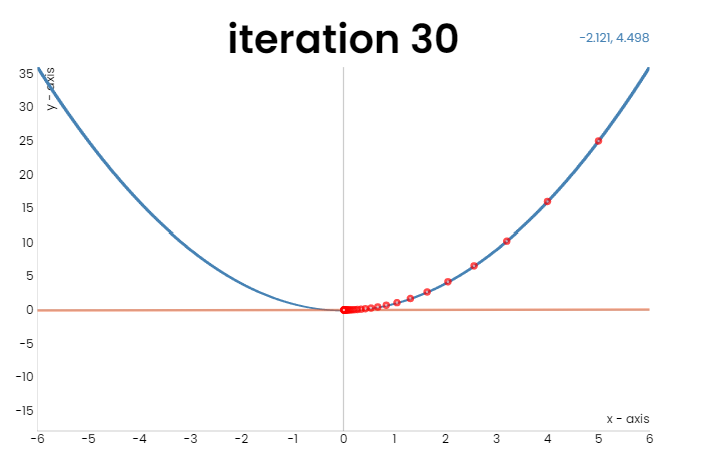
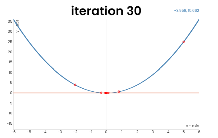
Figure 1: GD over \(f(x)=x^2\). Left: learning rate = 0.1; right: learning rate = 0.7.

In the figure above, we run GD over a quadratic function \(f(w)=w^2\), and one can see that GD indeed converges to the global minimum. However, GD suffers from the following problem: when the learning rate is small (the left figure), \(w_t\) consistently marches towards the global minimum \(0\), but the step size is small; when the learning rate is large (the right figure), the step size is large and the convergence is faster, but the trajectory oscillates, which makes the update ineffective. Gradient descent with momentum (GDM, also called Polyak’s heavy ball), is proposed to tackle this drawback. The intuition of GDM is simple: oscillatory trajectory is rooted from oscillatory gradient. Therefore, if we replace the gradient in the update of GD by an average of gradients of the past iterations, the oscillation will cancel out and the convergence should be faster. A psedocode of GDM is given as follows:

Psedocode of GDM

Input: objective function f, initial point \(w_0\), number of iterations \(T\), learning rate \(\{\eta_1,\cdots,\eta_T\}\), momentum parameter \(\beta\)

\[m_{0}=0\]

For \(t=1\rightarrow T\):

    \(m_t=\beta m_{t-1}+(1-\beta)\nabla f(w_t)\)

     \(w_{t+1}=w_{t}-\eta_t m_t\)

Output: \(w_{T+1}\)

Note both in GD and GDM, there are pre-determined hyperparameters \(\{\eta_1,\cdots,\eta_T\}\) called the learning rates. Practical choices are constant, diminishing and cosine, etc. In the above figure, we have demonstrated the power of learning rates, i.e., proper learning rates make the convergence faster. One can either picks learning rates through Grid Search, or through the prior knowledge of the objective function: theoretical analysis suggests that the optimal learning rate is negatively correlated with the local curvature (i.e., the norm of the Hessian matrix) of the objective funtion. As we usually can not predict the change of curvature along the optimization process, pre-determined learning rates do not suffice to offer satisfactory speed of convergence. A natural thought is to adaptively choose \(\eta_t\) according to the curvature during the optimization process. There is the motivation of adaptive optimizers. As the curvature in deep learning is very expansive to calculate, most adaptive optimizers use gradient norm instead of the curvature to estimate adaptive learning rates.

AdaGrad is among the earliest adaptive optimizers, first propsed simutaneously by [Streeter & McMahan, 2010] and [Duchi et al., 2011]. Its update is very simple: at step \(t\), it calculates the sum of historical gradients \(\nu_t=\sum_{s=1}^t \nabla f(w_t)^2\), and use \(\frac{1}{\sqrt{\nu_t}}\) as the adaptive learning rate. The concrete psedo-code of AdaGrad is given as follows:

Psedocode of AdaGrad

Input: objective function \(f\), initial point \(w_0\), number of iterations \(T\), learning rate \(\eta\), initial conditioner \(\nu_0\)

For \(t=1\rightarrow T\):

    \(\nu_t=\nu_{t-1}+\nabla f(w_t)^2\)

    \(w_{t+1}=w_{t}-\frac{\eta}{\sqrt \nu_t} \nabla f(w_t)\)

Output: \(w_{T+1}\)

AdaGrad converges faster than GD over many pratical problems (see Figure 2 as an example). Note that in the above we say “a natural thought is to adaptively choose \(\eta_t\) according to the curvature during the optimization process”, but AdaGrad chooses the adaptive learning rate based on gradient. Why AdaGrad still outperforms GD？Recent experimental results show that the curvature and the gradient norm of neural networks actually have strong correlationship. We invite interesting readers to see [Zhang et al., 2019] for details.

Despite that AdaGrad outperforms GD, one may immediately observe that the adaptive learning rate \(\frac{\eta}{\sqrt \nu_t}\) is non-increasing. This is problematic since as long as there is a large gradient along the training process, the adaptive learning rate will become small thereafter and contradict the intuition to be “adaptive”. RMSProp was proposed in Hinton’s lecture notes () to overcome this problem: it adds exponentially decayed weights to each term in \(\nu_t\), which makes \(\nu_t\) no longer non-decreasing. The psedo-code is given as follows:

Psedocode of RMSProp

Input: objective function \(f\), initial point \(w_0\), number of iterations \(T\), learning rate \(\eta\), initial conditioner \(\nu_0\), conditioner parameter \(\beta_2\in [0,1)\)

For \(t=1\rightarrow T\):

    \(\nu_t=\beta_2\nu_{t-1}+(1-\beta_2)\nabla f(w_t)^2\)

    \(w_{t+1}=w_{t}-\frac{\eta}{\sqrt \nu_t} \nabla f(w_t)\)

Output: \(w_{T+1}\)

RMSProp achieves better performance than AdaGrad. Finally, note that using adaptive learning rate (AdaGrad, RMSProp) and using momentum (GDM) are two orthogonal ways to accelerate the convergence. A natural thought is to combine them and see if their advantages can superimposed. Such a methodology indeed works, and lead to currently dominate optimizer Adam.

Psedocode of Adam

Input: objective function \(f\), initial point \(w_0\), number of iterations \(T\), learning rate \(\eta\), initial conditioner \(\nu_0\), momentum parameter \(\beta_1\), conditioner parameter \(\beta_2\in [0,1)\)

For \(t=1\rightarrow T\):

    \(m_t=\beta_1 m_{t-1}+(1-\beta_1) \nabla f(w_t)\)

    \(\nu_t=\beta_2\nu_{t-1}+(1-\beta_2)\nabla f(w_t)^2\)

    \(w_{t+1}=w_{t}-\frac{\eta}{\sqrt \nu_t} m_t\)

Output: \(w_{T+1}\)

In deep learning practice, \(f\) is usually an \(n\)-sum function, i.e., \(f(w)=\frac {1}{n}\sum_{i=1}^n f_i(w)\), where each \(f_i\) stands for the objective function calculated from a data. Thus, calculating \(\nabla f\) requires the calculation of every \(\nabla f_i\). As \(n\) is typically large (for example, 50k in Cifar 10), the calculation of \(\nabla f\) is costly. To resolve this obstackle, we estimate \(\nabla f\) by the average of gradients of a random subset (called batch) of \(\{f_1,\cdots, f_n\}\). Specifically, at the \(t\)-th iteration and with batch size \(b\), we uniformly sample \(b\) elements \(\{f_{\tau_{t,1}},\cdots, f_{\tau_{t,b}}\}\) from \(\{f_1,\cdots,f_n\}\) without replacement and calculate the estimation of \(\nabla f\) as \(\nabla \tilde{f}(w)=\frac{1}{b} \sum_{i=1 }^b \nabla f_{\tau_{t,i}}(w)\). By replacing \(\nabla f(w)\) by \(\nabla \tilde{f}(w)\) in the forementioned algorithms, we derive their stochastic version. We provide the psedo-code of stochastic GD (SGD) as follows, while the stochastic versionof other optimizers can be derived similarly.

Psedocode of SGD

Input: objective function \(f\), initial point \(w_1\), number of iterations \(T\), learning rate \(\{\eta_1,\cdots,\eta_T\}\), batch size \(b\)

For \(t=1\rightarrow T\):

    Sample \(\{\tau_{t,1},\dots,\tau_{t,b}\}\) uniformly without replacement from \(\{1,\cdots,n\}\)

      \(w_{t+1}=w_{t}-\eta_t \frac{1}{b}\sum_{i=1}^b\nabla f_{\tau_{t,i}}(w_{t})\)

Output: \(w_{T+1}\)

Figure2: (Image 6, [Ruder, 2016]) The behaviour of the different optimizers.

With \(b<<N\), stochastic gradient greatly saves the computation burden of each iteration, and allows stochatic optimizers to perform a lot more iterations than their deterministic counterparts given the same computation resources. While a single iteration of stochatic optimizers may not reduce \(f\) as effeciently as an iteration of their deterministic versions, the additional iterations make them performs better with limited computation resources. Thus, stochatic optimizers are more widely adopted.

Moreover, stochastic gradient has an additional benefit: it can help the optimizer find the global minima. We will discuss this detailedly in the next section.

Optimization vs. Sampling

In the last section, we have shown that the best solution that deterministic first-order optimizers can provide are the saddle points. This is because these optimizers can only access gradients. It is possible to provide better solutions by utilizing derivatives higher order. However, such derivatives are conputationally expansive due to the huge number of parameters of deep learning models. Surprisingly, we can step beyond saddle points by using stochatic first-order derivatives. We show this by leveraging the connection between optimization and sampling.

Let us revisit the stochastic gradient descent (SGD) as an example. The update rule of SGD can be rewritten as

\[w_{t+1}=w_{t}-\eta_t \frac{1}{b}\sum_{i=1}^b\nabla f_{\tau_{t,i}}(w_{t})=w_{t}-\eta_t \frac{1}{n}\sum_{i=1}^n\nabla f_{i}(w_{t})+\\\quad\quad\quad\quad\quad\quad\quad\quad\quad\quad\quad\quad\quad \eta_t(\frac{1}{n}\sum_{i=1}^n\nabla f_{i}(w_{t})-\frac{1}{b}\sum_{i=1}^b\nabla f_{\tau_{t,i}}(w_{t})).\]

In the right-hand-side of the above equality, the first two terms exactly agree with the update rule of GD, and thus the last term can be treated as the noise adding GD to get SGD. We denote the covariance of \(\frac{1}{n}\sum_{i=1}^n\nabla f_{i}(w_{t})-\frac{1}{b}\sum_{i=1}^b\nabla f_{\tau_{t,i}}(w_{t})\) by \(\mathcal{C}(w_t)\) and approximate the noise as a gaussian noise with same covariance, i.e.,

\[w_{t+1}\approx w_{t}-\eta_t \frac{1}{n}\sum_{i=1}^n\nabla f_{i}(w_{t})+\eta_t\mathcal{N}(0,\mathcal{C}(w_t)).\]

To further simplify the problem, we assume the noise covariance is independent of \(w_t\) and is isotropic, i.e., \(\mathcal{C}(w_t)\equiv \lambda \mathbb{I}\). We also assume that we use constant learning rate, i.e, \(\eta_t\equiv \eta\). The update rule of SGD then concides with the unadjusted langevin algorithm in sampling. Theoretical analysis tells us with proper conditions, the distribution of \(w_t\) will converge to \(p(w)\propto e^{-\frac{2}{\eta \lambda} \frac{1}{n}\sum_{i=1}^n\nabla f_{i}(w)}\). One can easily observe that \(p(w)\) is high when \(\frac{1}{n}\sum_{i=1}^n\nabla f_{i}(w)\) is small, and when \(w\) is the global minima, \(p(w)\) is largest. In other word, the global minima has the highest density, and thus SGD drives us to the global minima.

In general, optimization and sampling have deep connections. On the one hand, setting sampling density reversely proportional to the objective function and using sampling algorithms solve the optimization problem. On the other hand, acceleration techniques in optimization has inspired more effcient sampling algorithms.

Interface between Optimization and Generalization in Deep Learning: Implicit Regularization

While derived through optimization over the training data, learning models are often applied to unseen data. There is a natural gap between the performance over the training data and that over the unseen data, which is called the generalization error. By classical generalization theory, the generalization error grows with the model complexity, which further correlates with the model parameters. However, experiments show that the generalization error of deep learning model decreases when the number of parameter increases (called the “scaling law”). Therefore, classical generalization theory fail to explain the generalization ability of deep learning models and calls for new explxxnations. A potential approach is through the implicit regularization of optimizers: in classical generalization theory, the model complexity measures the complexity of models with nearly all possible parameter choices. However, the models output by the optimizers are only a small fraction of forementioned models and are with certain properties. The complexity of such models may not increase with the number of parameters. In other words, optimizers implicitly regularize the models to low model complexity. We illustrate this idea through the following theorem.

Theorem. Consider the linear classification problem. Let the data be separable, that is, there exists a linear model that can classify all data correctly. Then, the model output by GD has the largest \(L^2\) margin.

\(L^2\) margin has been proved to be positively correlate with the generalization error, and thus the above theorem indicate that GD implicitly regularize the model to possess good generalization ability. The above theorem has been extended to deep neural networks, and there are also other implicit regularization effect in deep learning. We invite the readers to see [Lyu & Li, 2019] for details.

References

Matthew Streeter and H Brendan McMahan, Less Regret via Online Conditioning, 2010

John Duchi, Elad Hazan, Yoram Singer, Adaptive Subgradient Methods for Online Learning and Stochastic Optimization, 2011

Sebastian Ruder, An overview of gradient descent optimization algorithms, 2016

Kaifeng Lyu, Jian Li, Gradient Descent Maximizes the Margin of Homogeneous Neural Networks, 2019

Jingzhao Zhang, Tianxing He, Suvrit Sra, Ali Jadbabaie, Why gradient clipping accelerates training: A theoretical justification for adaptivity, 2019