Author(s): Hong-Zhou Ye is currently a postdoctoral research scientist at Columbia University, working with Prof. Timothy C. Berkelbach on the development and application of highly accurate electronic structure theories to tackle complex chemistry challenges in condensed-phase systems. Hong-Zhou received his Ph.D. in chemistry from Massachusetts Institute of Technology (MIT), where he worked with Prof. Troy Van Voorhis on quantum embedding theory and methods for electronic excitations. Starting in the fall of 2024, Hong-Zhou will begin his independent career as an Assistant Professor of Chemistry at the University of Maryland (UMD). The Ye research group will be committed to leveraging theory and computational modeling to investigate intricate quantum phenomena in both molecules and condensed-phase materials, by combining existing wisdoms in quantum chemistry with recent developments in condensed-matter physics and artificial intelligence.

Chenru Duan is currently a research scientist at Microsoft Azure Quantum, working on building machine learning and quantum solutions for chemistry and materials industry. Chenru received his Ph.D. in chemistry from Massachusetts Institute of Technology (MIT), where he worked with Prof. Heather J. Kulik on AI applications in chemistry, building the first set of AI decision-making models and integrating them in high throughput computation, boosting the efficiency and accuracy for AI+computation centered chemical discovery. Chenru is a core member of AI4Science series workshop organizors and co-organizer the AI4Science workshop ICML2022, NeurIPS2022 and NeurIPS2023.

AI4Science101-Quantum Chemistry

What is quantum chemsitry?

A water molecule looks so much different from a protein molecule or a diamond crystal, but mathematically they are all the same: a set of positively charged nuclei being “glued” through Coulomb interaction by a set of negatively charged electrons. The electron “glue” is known as chemical bonds. In a nutshell, chemistry is the study and use of the electron “glue” to make new chemical species of desired properties. Quantum chemistry - often also known as electronic structure theory - aims to understand the electron “glue” itself using quantum mechanics.

The core of quantum chemistry is to solve the time-independent Schrödinger equation for electrons, \(H \Psi_n = E_n \Psi_n\), which is an eigenvalue problem for the electronic Hamiltonian \(H\) that defines a chemical system. The eigenfunction \(\Psi_n\) is the system’s wavefunction and the eigenvalue \(E_n\) is the associated energy, with the lowest-energy solution, denoted by \(\Psi_0\), being called the “ground” state and all others the “excited” states. In this article, we will mostly focus on solving for the ground-state wavefunction \(\Psi_0\) and its energy \(E_0\) (from now on we will occasionally omit the subscript “0”), the knowledge of which provides key information for understanding many physical and chemical properties of a molecule or a material. For example,

Knowing the energy of the reactant and the product in a chemical reaction allows calculating the reaction energy, while knowing how the energy responds to external parameters provides access to atomic forces, dipole moments, and polarizabilities, to name a few, of a molecule.
Knowledge of the wavefunction enables analyzing the orbitals, electron densities, electron correlation and entanglement, etc., all of which help provide a microscopic understanding of a chemical system.

Despite all the promises it makes, the Schrödinger equation for a general chemical system containing many electrons is computationally very challenging to solve. As we will see soon, the cost of obtaining an exact solution grows exponentially with the system size, and approximate solutions must be sought for in practice. Thus, the thesis of quantum chemistry is making approximations that balance accuracy and computational cost. This is exactly where recent developments in the machine learning (ML) community has stepped in and shown a great potential of addressing some perspectives of this challenge. In the rest of this article, we will first introduce basic context of quantum chemistry, followed by outlining recent progress in ML. We believe that this article will make quantum chemistry and ML research more accessible to readers from diversified backgrounds.

Dive in to quantum chemistry

This section is designed to offer a tailored introduction to quantum chemistry for readers who are familiar with linear algebra and probability theory but may not be well-versed in quantum mechanics. We begin with introducing some basic concepts of quantum chemistry, including variational principle, orbitals, and Hartree-Fock theory. This is followed by a survey of methods for electron correlation that can achieve “chemical accuracy”, with the goal of acquainting readers with many of the “buzz words” in quantum chemistry, such as DFT, CCSD(T), FCI, DMRG, QMC, to name a few. That’s quite a bit of information, so buckle up and let’s go!

For readers interested in diving deeper into quantum chemistry systematically, we recommend the classical textbook by Szabo and Ostlund, titled Modern Quantum Chemistry: Introduction to Advanced Electronic Structure Theory. We believe that the materials presented below serve as a good preview.

Basic concepts of quantum chemistry

Electronic Hamiltonian. The electronic Hamiltonian \(H\) includes all energy components related to the electrons in a molecule or material. For an \(N\)-electron system, \(H\) has two major contributions: the sum of individual electron Hamiltonians and the pairwise Coulomb interactions between electrons, i.e.,

\[H(x_1,\cdots,x_N) = \sum_{i=1}^{N} h(x_i) + \frac{1}{2} \sum_{i \neq j}^{N} v(x_i,x_j)\]

The specific forms of \(h\) and \(v\) are not crucial for our discussion below. However, it’s worth noting that \(h\) includes the Coulomb attraction between an electron and the nuclei, which introduces a parametric dependence of the full Hamiltonian \(H\) on the atomic coordinates \(R\). Solving the Schrödinger equation for various atomic configurations yields an energy profile as a function of these coordinates, denoted as \(E(R)\). This energy profile is commonly referred to as the “potential energy surface” and its derivatives \(\nabla_{R} E\) give the atomic forces, forming the basis for molecular dynamics, a topic discussed in a previous post on our blog.

Wavefunction is probability amplitude. God does play dice, and her dice is wavefunction. For an \(N\)-electron system, the probability density of simultaneously finding electron 1 at position \(x_1\), electron 2 at position \(x_2\), etc. is

\[\rho(X) = |\Psi(X)|^2\]

with the normalization condition

\[\int \mathrm{d}^N X\, |\Psi(X)|^2 = 1\]

where \(X = (x_1,\cdots,x_N)\). For this reason, wavefunction is a probability amplitude that encodes the correlation between electrons. Many properties of a molecule or a material can be calculated directly from its wavefunction as an expectation

\[A = \int \mathrm{d}^N X\, |\Psi(X)|^2 A(X) \equiv \langle \Psi | A | \Psi \rangle\] \[\langle \Psi |\cdot| \Psi\rangle\]

where the “bra-ket” notation

\[\langle \Psi |\cdot| \Psi\rangle\]

is due to Dirac. An relevant example for the discussion below is that the energy is an expectation of the Hamiltonian,

\[E = \langle \Psi | H | \Psi\rangle\]

Variational principle. A powerful tool to guide the construction of approximate wavefunction is variational principle, which states that the energy of any inexact “trial” wavefunction \(\tilde{\Psi}\) is no lower than the ground-state energy, i.e.,

\[E[\tilde{\Psi}] = \langle \tilde{\Psi} | H | \tilde{\Psi} \rangle \geq E_0\]

where the equality is taken if and only if \(\tilde{\Psi} = \Psi_0\). This theorem allows us to optimize an approximate wavefunction by minimizing its energy, a point we will frequently return to later.

Slater determinants. In an imaginary world where electrons do not interact, i.e., with the following non-interacting Hamiltonian

\[H_{\mathrm{NI}} = \sum_{i = 1}^{N} h(x_i)\]

the Schrödinger equation is solved by a Slater determinant

\[\Phi(X) \equiv \Phi(x_1,\cdots,x_N) = \frac{1}{\sqrt{N!} } \begin{vmatrix} \phi_1(x_1) & \cdots & \phi_1(x_N) \\ \vdots & \ddots & \vdots \\ \phi_N(x_1) & \cdots & \phi_N(x_N) \end{vmatrix}\]

where the one-electron wavefunction, aka orbitals, \(\{\phi_i\}\) are solutions to the one-electron Schrödinger equation

\[h(x) \phi_i(x) = \epsilon_i \phi_i(x)\]

with the eigenvalues \(\{\epsilon_i\}\) the orbital energies (which also form the energy bands in crystalline solids).

Readers familiar with probability theory may find the Hartree product, \(\Phi_{\mathrm{H}}(X) = \prod_{i=1}^{N} \phi_i(x_i)\), be their first guess for a non-interacting wavefunction. Indeed, one can show that the Slater determinant arises from antisymmetrizing the Hartree product, \(\Phi(X) = \mathcal{A} [\Phi_{\mathrm{H}}](X)\), where \(\mathcal{A}[f](x_1,x_2) = -\mathcal{A}[f](x_2,x_1)\). The reason behind this can be traced back to the Pauli exclusion principle, which states that the interchange of any electron pair leads to a change in the wavefunction’s sign. The distinction between \(\Phi\) and \(\Phi_{\mathrm{H}}\) is called the exchange effect, which is purely a quantum phenomenon. We will revisit this concept when discussing density functional theory (DFT) later.

Orbitals. In practice, the one-electron Schrödinger equation can be solved by expanding the unknown orbitals \(\phi_i(x)\) in a known set of \(K\) basis functions \(\chi_{\mu}(x)\) as \(\phi_i(x) = \sum_{\mu}^{K} c_{\mu i} \chi_{\mu}(x)\), turning the Schrödinger equation into a (Hermitian) matrix eigenvalue problem

\(\sum_{\nu}^{K} h_{\mu\nu} c_{\nu i} = \epsilon_i c_{\mu i}\) ( where \(h_{\mu\nu} = \langle \chi_{\mu} | h | \chi_{\nu} \rangle\) )

which can be solved readily by e.g., scipy.linalg.eigh. In almost all cases, we have \(K > N\) to minimize the basis incompleteness error. This leads to the concept of occupied and unoccupied orbitals.

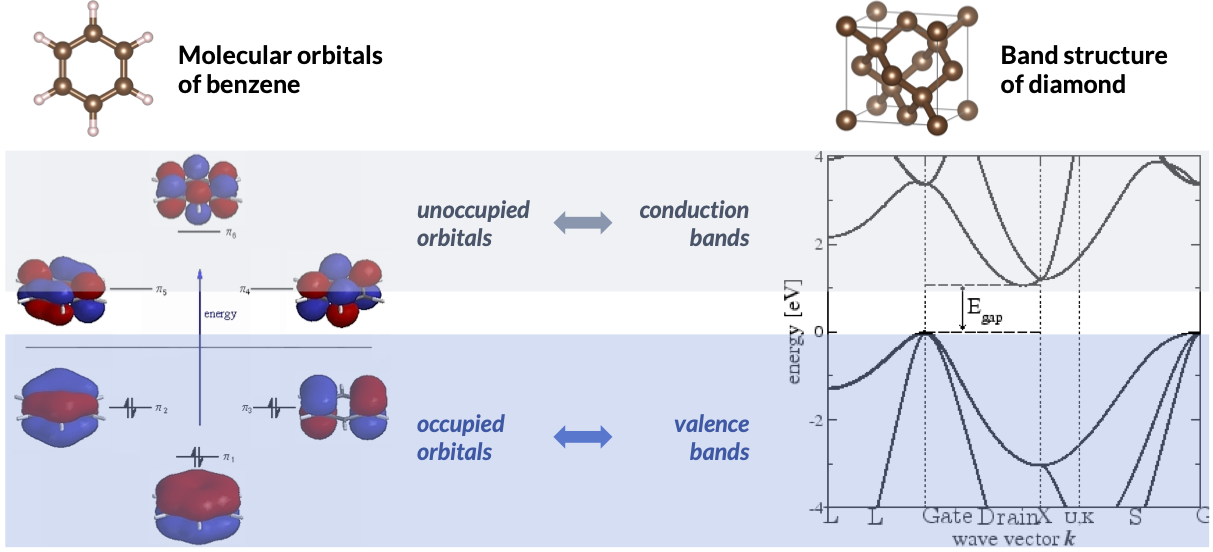
In the figure on the left, we show the valence orbitals and the corresponding orbital energy diagram for a benzene molecule generated using a minimal set of 6 basis functions. In the non-interacting ground-state \(\Phi_0\), the 6 valence electrons occupy the 3 orbitals with lowest energy. This is the theoretical foundation of the well-known picture where electrons in a molecule fill in the orbitals by their energy from low to high. The remaining 3 unoccupied orbitals do not contribute to \(\Phi_0\) but will become important in the correlated wavefunction theories that we will explore later. In the figure on the right, we show the orbital energy diagram for the diamond crystal. Here, the crystalline orbitals can be organized by symmetry labels of the crystal, and their orbital energy collectively forms what we known as energy bands. The occupied and unoccupied bands are often referred to as valence and conduction bands, respectively.

Of particular interest are the “frontier” orbitals located near the energy gap between the occupied and unoccupied manifolds. For example, the highest occupied and the lowest unoccupied molecular orbitals, i.e., HOMO and LUMO, are often the most active orbitals in a chemical reaction. Their counterparts in materials, the valence band maximum (VBM) and the conduction band minimum (CBM), determine the band gap and the effective mass for electron and hole transport.

We won’t delve into specifics here, but it’s worth noting that the basis functions \(\{\chi_{\mu}\}\) used to expand the orbitals are commonly referred to as Gaussian basis sets or atomic orbitals in molecular calculations and as plane waves in materials. Gaussian basis sets come in various flavors, often denoted by acronyms (e.g., 6-311G**, cc-pVTZ, def2-QZVPP, etc), while the plane-wave basis is characterized by a single parameter, its kinetic energy cutoff.

Hartree-Fock (HF) theory. Now going back to the physical world where electrons do interact, the single-determinant wavefunction \(\Phi\) is not exact anymore, but we can nonetheless use it as a trial wavefunction and apply variational principle. This leads to the Hartree-Fock (HF) theory with the following effective one-electron Schrödinger equation

\[F[\{\phi_i\}](x) \phi_i(x) = \epsilon_i \phi_i(x)\]

where the Fock operator \(F[\{\phi_i\}] = h + v_{\mathrm{HF}}[\{\phi_i\}]\) replaces the bare one-electron Hamiltonian \(h\). Like in the non-interacting case, the HF equation can be turned into a matrix eigenvalue problem by introducing a basis, and the picture where electrons fill in orbitals by energy discussed above still holds. However, two new features are worth some words.

The actual Coulomb potential \(v(x_1,x_2)\) in the HF theory is replaced by an effective Coulomb potential, \(v_{\mathrm{HF}}(x)\), averaged over all other \(N-1\) electrons. This is why HF is often referred to as the mean-field approximation.
The Fock operator that needs to be diagonalized depends on its own eigenfunctions (i.e., orbitals), which necessitates the iterative solution of the HF equation until self-consistency is achieved. This is why HF is also often referred to as the self-consistent field (SCF) theory.

A shocking fact about the HF theory is that it recovers > 99% of the total energy of a molecule or a material (Similar to the accuracy that you will get by plugging in a naive CNN to the MNIST dataset)! For this reason, HF provides a decent qualitative description for most chemistry problems. However, getting the remaining 1% correctly is what really makes a theory quantitative and predictive. The reason here is about relevant energy scales: the total energy of a molecule is often hundreds or even thousands of Hartree, while chemical reactions occur on the scale of kcal/mol (1 Hartree ≈ 630 kcal/mol). In quantum chemistry, people often refer 1 kcal/mol as “chemical accuracy.” In the next subsection, we will introduce theories that are capable of achieving this level of precision, which form the core of quantum chemistry.

It is interesting to note that one of Google’s “quantum computing for quantum chemistry” papers implemented exactly the HF theory on a quantum computer and used it to study a simple reaction. Now you know (the chemistry part of) what they were doing!

Methods for electron correlation

Overview. Two primary strategies exist for going beyond the HF mean-field approach. Correlated wavefunction theories employ a more sophisticated wavefunction ansatz than the HF single Slater determinant. In contrast, density functional theory (DFT) – in its most widely used Kohn-Sham (KS) formulation – retains the single determinantal wavefunction but alters the HF potential into a KS potential that accounts for electron correlation effects. Both approaches have their strengths and weaknesses, which can potentially be harnesses or addressed through integration with ML. We believe that having a fundamental grasp of each of these methods is essential for achieving this goal.

Density functional theory (DFT). Up to this point, our discussion has primarily revolved around wavefunctions. However, an alternative formalism was introduced by Hohenberg and Kohn (HK) in 1964, who demonstrated that the electron density

\[\rho(x) = \int \mathrm{d}x_2\cdots\mathrm{d}x_{N}\, |\Psi(x,x_2,\cdots,x_N)|^2\]

could serve as the fundamental quantity instead. Specifically, HK proved two mathematical theorems about \(\rho(x)\):

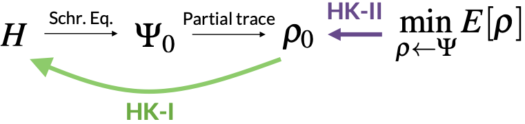
The first theorem (HK-I) establishes the equivalence between \(\rho\) and \(\Psi\) by proving that given a system’s electron density, one can uniquely determine the Hamiltonian (up to a constant energy shift) and hence in principle, determine the wavefunction.
The second theorem (HK-II) establishes a variational principle for \(\rho\) by showing that the ground-state electron density \(\rho_0\) minimizes the energy functional \(E[\rho]\), i.e., just like \(\Psi_0\) minimizing \(E[\Psi]\).

Unfortunately, the precise expression for \(E[\rho]\) remains unknown. However, HK theorems provide a valuable decomposition of \(E[\rho]\), as follows:

\[E[\rho] = \int\mathrm{d}x\, \rho(x) v_{\mathrm{ext}}(x) + F[\rho]\]

Here, the first term accounts for the energy resulting from the external potential that is system-dependent (e.g., the nuclear potential in a molecule), while the second term, known as the universal energy functional, encompasses all the electron-electron interaction and is universal for all molecules and materials for their ground-state properties.

Kohn-Sham (KS)-DFT. At the heart of DFT lies the quest for practical approximations to \(F[\rho]\). Thus far, the most popular variant is KS-DFT, where one aims to construct a non-interacting system – described by a Hartree product \(\Phi_{\mathrm{H}}\) – whose electron density is equal to the exact ground-state density \(\rho_0\). The KS energy functional is

\[E_{\mathrm{KS}}[\rho] = \langle\Phi_{\mathrm{H}}|H|\Phi_{\mathrm{H}}\rangle + E_{\mathrm{xc}}[\rho] = \sum_{i} \langle\phi_i|h|\phi_i\rangle + J[\rho] + E_{\mathrm{xc}}[\rho]\]

In the second equality, the first term is simply a sum of one-electron energy and the second term is the classical electrostatic energy which includes self-interaction. The last term, known as the exchange-correlation (xc) functional, encapsulates the missing exchange and electron correlation effects and necessitates practical approximation. On initial inspection, it might seem like this rewriting doesn’t solve any problem: the exact form of \(E_{\mathrm{xc}}[\rho]\) remains elusive. Nevertheless, the KS approach proves effective because \(E_{\mathrm{xc}}[\rho]\) is relatively small in magnitude (similar to the correlation energy). Consequently, it can be reasonably approximated in practice.

Applying variational principle, i.e., making \(E_{\mathrm{KS}}[\rho]\) stationary w.r.t the underlying orbitals leads to the KS equation

\[F_{\mathrm{KS}}[\rho](x) \phi_i(x) = \epsilon_i \phi_i(x)\]

where the KS operator, \(F_{\mathrm{KS}}[\rho] \equiv \delta E_{\mathrm{KS}}[\rho] / \delta \rho = h + v_{J}[\rho] + v_{\mathrm{xc}}[\rho]\), parallels the Fock operator in HF theory. The KS equation can be solved in a manner analogous to solving the HF equation, with the \(\rho\)-dependence of the KS operator also necessitating an iterative approach to achieve self-consistency. Similar to HF, KS-DFT is an effective one-electron theory where the quantum (i.e., exchange) and many-body (i.e., correlation) effects of electrons are encapsulated in the xc potential, \(v_{\mathrm{xc}}[\rho] = \delta E_{\mathrm{xc}}[\rho] / \delta \rho\). This renders KS-DFT rather convenient because it preserves all the one-electron concepts discussed earlier, including HOMO/LUMO, energy bands, etc.

The “Jacob’s Ladder” of KS-DFT. Different approximations to \(E_{\mathrm{xc}}[\rho]\) define the “level of theory” in KS-DFT. Define the xc energy density \(\varepsilon_{\mathrm{xc}}[\rho](x)\) as in

\[E_{\mathrm{xc}}[\rho] = \int \mathrm{d}x\, \rho(x) \varepsilon_{\mathrm{xc}}[\rho](x)\]

There are three classes of “pure” DFT methods where \(\varepsilon_{\mathrm{xc}}[\rho](x)\) is a local function (i.e., not a functional) as in

\[E_{\mathrm{xc}}^{\mathrm{pure}}[\rho] = \int \mathrm{d}x\, \rho(x) \varepsilon_{\mathrm{xc}}(x)\]

Local density approximation (LDA), where \(\varepsilon^{\mathrm{LDA}}_{\mathrm{xc}}(x) = \varepsilon_{\mathrm{xc}}(\rho(x))\) depends only on the local electron density \(\rho(x)\).
Generalized gradient approximation (GGA), where \(\varepsilon_{\mathrm{xc}}^{\mathrm{GGA}}(x) = \varepsilon_{\mathrm{xc}}(\rho(x),\nabla\rho(x))\) further depends on the local density gradient \(\nabla \rho(x)\).
meta-GGA, where \(\varepsilon_{\mathrm{xc}}^{\mathrm{mGGA}}(x) = \varepsilon_{\mathrm{xc}}(\rho(x),\nabla\rho(x),\tau(x))\) further depends on the kinetic energy density, \(\tau(x)\).

There are also “hybrid” DFT methods where the xc functional has explicit dependence on orbitals:

Hybrid DFT, where the exchange part of \(E_{\mathrm{xc}}[\rho]\) is a mixture of a pure exchange functional and the HF exchange, which depends on the occupied orbitals, \(E_{\mathrm{xc}}^{\mathrm{hyb}}[\{\phi_i\}_{i=1}^{N}] = (1-a) E_{\mathrm{x}}^{\mathrm{pure}}[\rho] + a E_{\mathrm{x}}^{\mathrm{HF}}[\{\phi_i\}_{i=1}^{N}] + E_{\mathrm{c}}^{\mathrm{pure}}[\rho]\).
Double-hybrid DFT, where the correlation part of \(E_{\mathrm{xc}}[\rho]\) is also mixed with the correlation energy from some correlated wavefunction theory, which depends on both the occupied and the virtual orbitals, \(E_{\mathrm{xc}}^{\textrm{double-hyb}}[\{\phi_i\}_{i=1}^{K}] = E_{\mathrm{x}}^{\mathrm{hyb}}[\{\phi_i\}_{i=1}^{N}] + (1-b)E_{\mathrm{c}}^{\mathrm{pure}}[\rho] + b E_{\mathrm{c}}^{\mathrm{WFT}}[\{\phi_i\}_{i=1}^{K}]\).

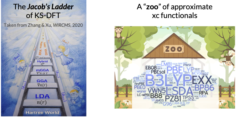
The five approximate classes together form a hierarchy of KS-DFT that is termed the “Jacob’s ladder” by John Perdew. Higher accuracy is obtained in general as we ascend the ladder, at the price of a higher computational cost. Specifically, pure DFT has a cost scaling of \(O(N^3)\), hybrid DFT (comparable to HF) has a scaling of \(O(N^4)\), and commonly used double-hybrid DFT, which is based on MP2 or the closely related random-phase approximation (RPA), scales as \(O(N^5)\). There are a few hundreds of xc functionals available in the Libxc library, making a “zoo” of KS-DFT methods. Some widely used xc functionals are PBE (a GGA), B3LYP (a hybrid GGA), and M06-2X (a hybrid meta-GGA), to name a few. Recent developments include self-interaction correction (SIC), range-separated hybrid (RSH), and dispersion correction (e.g., DFT-D). A comprehensive benchmark of xc functionals for chemical problems can be found here. Despite hundreds of xc functionals have been developed, none of them is universally accurate across the entire chemical space, motivating a Tiktok-like recommender approach of matching chemical systems and their “best-performing” xc functionals, as will be discussed later in the Navigating through the zoo of density functional section.

Developing an xc functional. Finally, we give a brief overview on how xc functionals are developed. There are two major strategies:

The physics-driven or non-empirical strategy employs functional forms that satisfy known mathematical constraints the exact functional must obey (see here for a review). The most famous example is perhaps the Perdew-Burke-Ernzerhof (PBE) GGA functional, which satisfies 11 constraints. A more recent development is the strongly-constrained and appropriately-normed (SCAN) meta-GGA functional, which satisfies all 17 known constraints that a meta-GGA functional can satisfy.
The data-driven or semi-empirical strategy employes a flexible functional form (usually a power series) with undetermined parameters and fits the parameters to accurate reference data, such as CCSD(T) results on small molecules. The most well-known example in this category is perhaps the Minnesota family, which consists of nearly 20 highly-parameterized functionals published by the Trular group since 2005. For example, the MN15 functional has a total of 59 fitted parameters.

The distinction between the two “schools” of functional design is not absolute, and many semi-empirical functionals also include parameters that are determined by satisfying known exact constraints. Indeed, many of the most successful “chemists’ xc functionals” are developed this way, including BLYP, B3LYP, and more recently, the “combinatorially optimized” \(\omega\)B97X functional. The data-driven nature also renders ML a natural choice for functional design. A recent example of success in this direction is the deep neural network-based DM21 functional developed by DeepMind.

For readers interested in learning DFT more systematically, we recommend Burke’s website, which features an introductory textbook titled The ABC of DFT and an extensive collection of review articles. This compilation also includes resources on time-dependent DFT for excited states, a topic that we have not covered in this article.

Correlated wavefunction theories. Different correlated wavefunction theories differ in two ways: (i) how the wavefunction is parameterized (i.e., what the ansatz is), and (ii) how the parameters are determined. The former gives rise to different families of correlated wavefunction methods such as configuration interaction (CI), coupled cluster (CC), quantum Monte Carlo (QMC), and many more. The latter determines if a method is variational or perturbative, or is deterministic or stochastic.

Variational methods: CI, DMRG, and VMC. The first class of methods we introduce are based on the variational principle that we briefly discussed above. Let \(\Psi(\vec{c})\) depend on some parameters \(\vec{c}\), which makes the energy a function of these parameters as well

\[E(\vec{c}) = \langle\Psi(\vec{c})|H|\Psi(\vec{c})\rangle\]

By variational principle, \(E(\vec{c}) \geq E_0\) (the true ground-state energy) for all \(\vec{c}\), and we can optimize our wavefunction by minimizing its energy

\(\vec{c} \gets \min_{\vec{c}} E(\vec{c})\).

All variational methods share the following two computational advantages.

The energy is an upper bound of the exact ground-state energy, which can often be used as a means to gauge the quality of a wavefunction form.
The energy obeys the Hellmann-Feynman theorem, which simplifies the calculation of energy derivatives (e.g., atomic forces).

Different variational methods differ by the specific wavefunction ansatze being used.

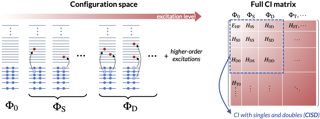
Full configuration interaction (FCI). Recall that we solve the one-electron Schrödinger equation (and the HF equation) by introducing a set of \(K\) basis functions and transforming it into a matrix eigenvalue problem of size \(K^2\). The same approach can be applied to solve an \(N\)-electron Schrödinger equation – if we can find a proper \(N\)-electron basis set! A legitimate choice is all \(K \choose N\) determinants one can obtain by populating the \(K\) HF orbitals with \(N\) electrons. The HF determinant \(\Phi_0\) has the lowest energy and is called the ground-state configuration. Promoting electrons from the HF occupied orbitals to the unoccupied ones leads to excited-state configurations that can be classified as single (S), double (D), triple (T), etc. excitations, based on how many electrons are excited from \(\Phi_0\). The full configuration interaction (FCI) wavefunction is a linear combination of all configurations \(\Psi_{\mathrm{FCI}} = \sum_{I} c_{I} \Phi_{\mathrm{I}} = c_0 \Phi_0 + c_{\mathrm{S}} \Phi_{\mathrm{S}} + c_{\mathrm{D}} \Phi_{\mathrm{D}} + c_{\mathrm{T}} \Phi_{\mathrm{T}} + \cdots\) This transforms the \(N\)-electron Schrödinger equation into a gigantic matrix eigenvalue problem of size \({K \choose N}^2\), solving which results in the exact solution to the \(N\)-electron Schrödinger equation within the chosen one-electron basis set. Since the dimension of the FCI problem \(K \choose N\) grows exponentially with both \(K\) and \(N\), we say that FCI has an exponential computational scaling. In practice, FCI is limited to systems with up to 20 electrons, but nonetheless serves as the absolute reference for benchmarking more approximate methods on small molecules.
Truncated CI. Restricting the FCI expansion to a subset of configurations gives the truncated CI theory, which is the most straightforward approximation to FCI. For example, a CI with singles and doubles (CISD) wavefunction is \(\Psi_{\mathrm{CISD}} = \sum_{I} c_{I} \Phi_{\mathrm{I}} = c_0 \Phi_0 + c_{\mathrm{S}} \Phi_{\mathrm{S}} + c_{\mathrm{D}} \Phi_{\mathrm{D}}\) Following the same logic, there is a hierarchy of truncated CI methods, CISD (\(N^6\)), CISDT (\(N^8\)), CISDTQ (\(N^{10}\)), and so on, which systematically approaches FCI. However, truncated CI is not commonly used in quantum chemistry these days due to its violation of size-consistency, a point that will become clear below when discussing perturbation theory.

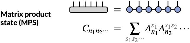
Tensor networks. An alternative to parameterizing the CI expansion is tensor networks, exemplified by the density matrix renormalization group (DMRG) method. The tensor networks theory is motivated by the second-quantization formulation of quantum mechanics, in which the FCI expansion can be written as \(\Psi_{\mathrm{FCI}} = \sum_{n_1,n_2,\cdots} C_{n_1n_2\cdots} |n_1,n_2,\cdots\rangle\) where \(|n_1,n_2,\cdots\rangle\) is a Slater determinant with \(n_1\) electron(s) in orbital 1, \(n_2\) electron(s) in orbital 2, and so on. Here, the key observation is that the coefficients \(C_{n_1n_2\cdots}\) are elements of a high-dimensional tensor. Similar to how a matrix can possess a low-rank structure that can be exploited using algorithms such as the singular value decomposition (SVD), higher-dimensional tensors can also be broken down into products of tensors with lower dimensions or ranks, which is why they are termed “tensor networks.” In particular, DMRG employs a matrix product state (MPS) to approximate the coefficient tensor \(C_{n_1n_2n_3\cdots} \approx \sum_{s_1s_2s_3\cdots}^M A_{n_1}^{s_1} A_{n_2}^{s_1s_2} A_{n_3}^{s_2s_3} \cdots\) where the \(\mathbf{A}\) tensors are variational parameters. The DMRG wavefunction can be progressively improved to approach FCI by increasing the “bond dimension”, \(M\), which controls the rank of the product tensor. The cost scaling of DMRG is \(O(N^4)\) but the prefactor grows with bond dimension as \(O(M^3)\). Recent implementations have demonstrated the ability to attain FCI-level accuracy for about 80 electrons (see e.g., a recent preprint from the Chan group). Methods like DMRG thus significantly expand the scope for FCI-like methods.
Variational Monte Carlo (VMC). A major difficulty preventing one from using an arbitrary wavefunction ansatz in variational optimization is the high computational cost associated with evaluating the energy (and its gradients), which, when written explicitly, is a multi-dimensional integral explicitly

\[E[\Psi] = \frac{\int \mathrm{d} X |\Psi(X)|^2 H(X)} {\int \mathrm{d} X |\Psi(X)|^2}\]

Varitional Monte Carlo (VMC) bypasses this curse of dimensionality by using Monte Carlo sampling to stochastically evaluate the needed integrals. As a result, VMC enables using some wavefunction forms that are otherwise inaccessible to direct variational optimization. A commonly used one is the Slater-Jastrow ansatz

\[\Psi_{\mathrm{SJ}}(X) = \Phi_0(X) \exp\left[ \sum_{i < j} u_{ij}(x_i,x_j) \right]\]

where the Jastrow correlation factor \(u_{ij}\), being the variational degrees of freedom, explicitly encodes the correlation effect between two electrons. One disadvantage of VMC (and any other stochastic methods) is the inherent statistical error, which can complicate the evaluation of atomic forces and other properties.

Perturbation methods: MBPT and CC. While giving an energy upper bound by variational methods seems an appealing property, in practice what is often more important is size-consistency. A method is size-consistent if it predicts the energy of two non-interacting molecules to be the same as the sum of the energies of the two individual molecules, i.e., \(E(A+B) = E(A) + E(B)\). Methods violating size-consistency introduce bias based on system size, resulting in poor performance for e.g., reaction energy calculations. A closely related concept for condensed-phase materials is size-extensiveness. A method is size-extensive if the energy scales linearly with system size in the bulk limit, i.e., \(E(N) \propto N\) for \(N \to \infty\). Unfortunately, most variational methods are neither size-consistent nor size-extensive, rendering them unsuitable for simulating chemical reactions or condensed-phase systems in general. An important exception is FCI, which is both variational and size-consistent/extensive for the trivial reason that FCI being the exact solution. Consequently, variational methods are mostly used for generating highly accurate reference results for small molecules (or small active space in CAS methods) where one can reliably approach the FCI limit.

The above discussion motivates the introduction of many-body perturbation theory (MBPT) and coupled cluster (CC) theory, both of which are rigorously size-consistent and size-extensive and hence more applicable to large systems.

Many-body perturbation theory (MBPT). For systems where electron correlation is not strong, the HF ground state \(\Phi_0\) dominates the FCI expansion with \(c_0 \sim 1\). The remaining CI coefficients, being small in magnitude, can be determined in a perturbative manner. Mathematically, this is done by separating the Hamiltonian into two parts, \(H = F + V\), where the eigen spectrum of the Fock operator \(F\) is already known (\(\Phi_0, \Phi_{\mathrm{S}}, \Phi_{\mathrm{D}}, \cdots\)). The wavefunction and energy are then expanded as power series of the “fluctuation potential” \(V\) and can be solved for order by order. The leading order correction to the HF energy comes from double excitations and is at second order, resulting in the MP2 theory (named after its two original developers, Møller and Plesset). MP2 has been widely used in molecules and more recently in materials for its size-consistency/extensiveness and, perhaps more important, it being the cheapest correlated theories, with a modest \(O(N^5)\) computational scaling. MP2 is the first member of the MP\(n\) series, followed by MP3 (\(N^6\) cost), MP4 (\(N^7\) cost), and so on that include triple excitations and higher-order effects. However, these higher-order perturbation theories are not as commonly used as MP2 due to their slow convergence to FCI or, in some cases, divergence. Additionally, MP3 and higher-order methods share similar cost scalings with more powerful theories like coupled cluster, which we will introduce now.
Coupled cluster (CC). The CC wavefunction takes an exponential form \(\Psi_{\mathrm{CC}} = \mathrm{e}^{T} \Phi_0 = \left( 1 + T + \frac{1}{2}T^2 + \cdots \right) \Phi_0\) where \(T = T_1 + T_2 + \cdots\) generate single, double, etc. excitations from \(\Phi_0\). It can be shown that when \(T\) is untruncated, the full CC wavefunction is equivalent to FCI and hence exact. In practice, \(T\) is truncated to include only low-level excitations just like truncated CI. For example, \(T = T_1 + T_2\) gives coupled cluster with singles and doubles (CCSD). The cost scaling of CCSD is \(O(N^6)\) and equivalent to MP3 and CISD. However, CCSD has two key advantages that make it the most widely used \(O(N^6)\)-scaling method.
1. CCSD iteratively determines coefficients for the single (\(T_1\)) and double (\(T_2\)) excitations, encompassing their contributions to an infinite order. This is similar to CISD but much better than MP3, which is only correct up to the second order in double excitations (cf. MP2 is first order in double excitations).
2. The exponential form of the wavefunction generates products of excitations that correspond to disconnected higher-order excitations. For example, the simultaneous excitation of two distant electron pairs is important for electron correlation in large molecules or materials, but being a (disconnected) quadruple excitation means that it requires at least MP4 (\(\geq N^7\) cost) or CISDTQ (\(\geq N^8\) cost). By contrast, CCSD naturally includes this excitation type through the \(T_2^2\) term generated by expanding the exponential, as well as many more disconnected higher-order terms such as \(T_1 T_2\), \(T_1^2 T_2\), \(T_1 T_2^2\), etc.
For many chemistry problems where electron correlation is weak, CCSD can be further improved by perturbatively including the triple excitations, leading to one of the most successful correlated wavefunction theories in quantum chemistry, coupled cluster with singles, doubles, and perturbative triples [CCSD(T)]. CCSD(T) consistently delivers chemical accuracy for weakly correlated problems and is often dubbed the quantum chemistry “gold standard”. The \(O(N^7)\) cost scaling of CCSD(T) limits its application to small molecules of approximately 10 atoms, but various linear-scaling techniques, exemplified by the domain local pair natural orbitals (DLPNO) and local natural orbitals (LNO) approximation, have significantly expanded the scope of CCSD(T) to systems with up to 100 atoms. For example, in a recent work, Ye and Berkelbach employed a periodic implementation of LNO-CCSD(T) to study water dissociation on TiO2 surfaces.

For readers eager to learn MBPT and the CC theory systematically, especially the powerful diagrammatic tools that simplify the derivation of seemingly complex algebraic expressions, we recommend the textbook by Shavitt and Bartlett, titled Many-Body Methods in Chemistry and Physics: MBPT and Coupled-Cluster Theory.

Topics not covered here

The above only serves as an outline for a subset of quantum chemistry methods. Here’s a list of other developments you may find interesting.

Strongly correlated systems. The correlated wavefunction theories we’ve discussed are primarily categorized as “single-reference” methods, which operate under the assumption \(c_0 \approx 1\) in the FCI expansion, implying that HF already offers a reasonable starting point. Systems satisfying this criterion are often referred to as weakly correlated. This includes most closed-shell systems (which lack unpaired electrons) with a sizeable HOMO-LUMO/band gap. Classical examples include many organic molecules and simple insulating solids. On the other hand, strongly correlated systems are those where multiple configurations contribute significantly to the FCI wavefunction, meaning that \(c_0 \ll 1\). Such systems typically require multi-reference methods for an accurate description. Many single-reference methods have corresponding multi-reference extensions, such as complete active space self-consistent field (CASSCF), CAS perturbation theory to the second-order (CASPT2), multi-reference configuration interaction (MRCI), among others. Strongly correlated systems are often characterized by the presence of unpaired electrons, found in radical molecules and magnetic materials, or by a small energy gap. In this context, DFT behaves more like a mean-field approximation and often fails catastrophically when applied to strongly correlated systems.
Excited states. The discussion above is limited to the electronic ground states. Excited states, being higher-energy solutions to the Schrödinger equation, are crucial for understanding photochemistry and many physical processes in solids, such as excitons and plasmons. Two primary strategies exist for expanding a ground-state theory to simulate excited states. The direct approach involves directly seeking higher-energy solutions to the Schrödinger equation within the same approximation as the ground-state theory. The response approach, on the other hand, describes excited states as the response of the ground state to a time-dependent perturbation. Examples of the former category include ΔSCF (aka orbital-optimized DFT within the KS-DFT framework), state-specific/average CASSCF, while examples of the latter include time-dependent DFT (TDDFT), equation of motion CC (EOM-CC), among others. For an introductory review on excited-state methods, we recommend a 2005 Chemical Review article by Dreuw and Head-Gordon.

Recent advances with ML in quantum chemistry

Bypassing the need to solve the Schrödinger equation

It has been a while since 2013 that people use machine learning (ML) to predict chemical properties of molecules or the energy and forces for molecular dynamics, but these ML model do not really learn the foundamental electronic structures of the molecules and materials from a perspective of solving the Schrödinger equation and alike. However, there has been a recent surge of development where ML is directly baked in quantum chemistry, such as predicting the electron density, Hamiltonian matrix, and wavefunctions. These models have become increasingly accurate with the widespread of equivariant neural networks, which preserve all the symmetries required for these tensorial foundamental quantum chemistry properties (e.g., e3nn).

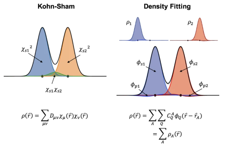
Predicting electron density.- Electron density is a fundamental variable in density functional theory (DFT), from which, in principle, all ground state properties can be derived. Therefore, it is the “to-go” target for chemistry and materials system beyond energy and forces. Well ahead of the rise of equivariant models, Grisafi et al. built a symmetry-adapted Gaussian process regression (SA-GPR) model to matain the correct symmetries that an ML model needs for electron density prediction. They found that, trained on short alkanes (CH4, C2H6, C3H8, …), SA-GPR can readily generalize to larger alkanes of different conformations. Besides enforcing the ML model to have the correct symmetry, many attemped to encode the symmetry in the molecular representation. For example, Achar et al. used Smooth Overlap of Atomic Positions (SOAP) as representation to learn the electron density for both molecular and materials systems. More recently, people have adapted density fitting, a conventional quantum chemistry approach to partition the total electron density to the single-atom basis,

\(\rho(r) = \sum_{\mu, \nu} D_{\mu \nu} \chi_\mu(r) \chi_\nu(r) = \sum_{A,Q} C_A^Q \phi_Q(r-r_A) = \sum_A \rho_A(r)\) which projects the original basis functions based electron density (with density matrix \(D_{\mu \nu}\)) to atom-centered auxilliary basis (\(C_A^Q\)). Therefore, with equivariant neural networks, we can directly learn these decomposed tensors from electron density, boosting both the model accuracy and transferability.

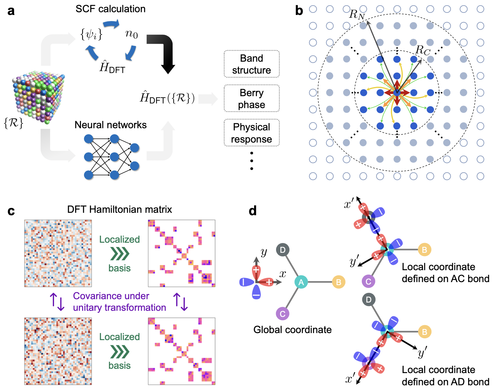
Predicting Hamiltonian matrix.- The goal of SCF calculations in DFT (or HF) is to obtain the converged Hamiltonian matrix as the solution of \(H_{DFT} \Psi = E \Psi\) in the non-interacting basis representation. Then almost all electron-related physical quantities in the single-particle picture can be derived, such as charge density, band structure, and physical responses to electromagnetic fields. Compared to electron density, \(H_{DFT}\) is practically more straightforward to derive these property. However, \(H_{DFT}\) is at the size of \(N^2\), where \(N\) is the number of basis function, which is too large to learn. Luckily, one can ultilize the principle of locality in normal chemical system (this assumption breaks down for “quantum matter” that has very strong correlation). Thus, there is no need to study the entire \(H_{DFT}\), but only its sparsed approximation, which then reduce the scaling to O(N). Combined with equivariant model architecture, Li et al. showed that they can learn the Hamiltonian quite accurately, even to a degree that unveils the band structure of bilayer twisted graphene.

Neural network as a functional approximator

Many complication in quantum chemistry boils down to the high-dimentional mapping between a system of study to its electronic structure properties, such as electron density and wavefunction. Therefore, a school of thought is to approximate this underlying mapping when we construct the solution.

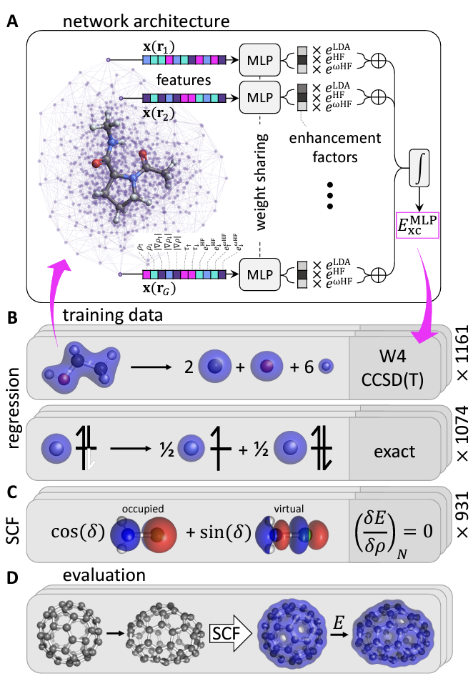
Neural network as a density functional.- The Kohn–Sham (KS) DFT, in which only the exchange-correlation (xc) energy needs to be approximated as a functional of the density, has greatly improved accuracy while “only” scales to \(O(N^3)\). Due to the approximation in xc functional, there would be errors that are somewhat unpredictable during its application. Once the exact xc was found, however, all ground-state properties would be solved in agreement with FCI at a \(O(N^3)\) cost, which is the dream of quantum chemistry. ML has already helped with functional development. Almost 20 years ago, using Bayesian inference, a new DFA can be assembled as a linear combination of functional forms with statistically inferred coefficients, accelerating DFA design using known functional forms and alleviating the risk of overfitting during DFA parameterization. ANNs have been used as an ansatz for designing DFAs due to their ability to represent any function. Brockherde et al. developed ML models that directly learn the ground-state density of a system, reducing the computational cost of solving the Kohn–Sham (KS) DFT equations iteratively. By incorporating the KS equations as a regularization term in the loss function and providing feedback to ANNs in each training iteration, Nagai et al. and Li et al. demonstrated that the ANN functional can be learned with very few training molecules. Kasim et al. recast KS-DFT in a fully differentiable framework, enabling a density functional expressed as an ANN to be optimized with backpropagation, which demonstrated transferability to other small molecules containing elements and bond types not in the training set. Again, with the widespread of open-source packages for equivariant neural networks, people have recently shifted towards including symmetries and exact constraints of the exact xc during learing density functional, with a prominent example as DM21, where the piece-wise linearilty and flat-plane condition were explicitly considered.

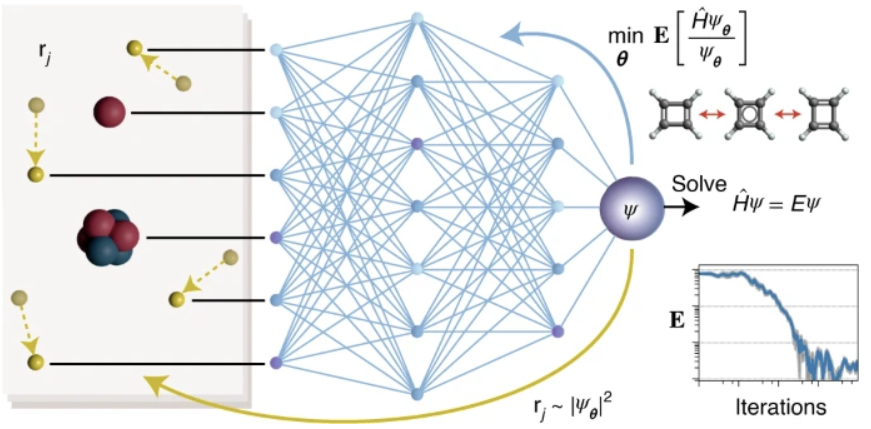
Neural network as ansatz in quantum Monte Carlo (QMC).- As a variantional approach, QMC has the great property that for whatever guess wavefunction, the resulting electronic energy will always smaller or equal (if the guess is the true wavefunction) to the ground state energy. Therefore, by modeling wave functions as NNs and using the resulting energy expectation as the loss function, one can employ self-consistently sampling from the square of the wave function with QMC and generates its own data on the fly. This approach has been applied to spin systems on lattices and Hubbard model. By modifying the ansatz to include anti-symmetry constraints, Hermann et al. parameterized a multi-determinant Slater-Jastrow-backflow type wavefunction with NN. By applying the variational principle on this ANN wavefunction ansatz, they showed that the correlation energy can be quickly recovered (ca. 99%) for most of their test systems using very few (i.e., 10) determinants. To date most approaches have only been demonstrated on small systems with paired electrons, where MR WFT calculations can be performed easily. It is imperative to extend these developments to large systems with challenging electronic structure (e.g., metal–organic bonding) in order to impact ML-accelerated discovery of novel materials.

Integrating ML models in high throughput computation

With the advancement of cloud infrastructure and workflow automation, high throughput computation (HTC), where thousands of jobs are simutaneously run under workflow management instead of one, has been a common tool to generate large databsets for chemical and materials discovery. Despite there are so many quantum chemistry methods out in the market, DFT remains the most accurate method among all that are practical (e.g., force field, semi-emperical) in HTC. However, the accuracy of DFT depends on the choice of density functional. That is where ML can help.

Addressing DFT sensitivity.- Density functionals are conventionally selected based on intuition or computational cost, thus introducing bias in data generation and reducing the quality of the data in a way that degrades utility for discovery efforts. To address this challenge, McAnanama-Brereton and Waller developed an approach to identify optimal DFA-basis set combinations using game theory. They devised a three-player game addressing accuracy, complexity, and similarity of DFA-basis set combinations and solved the Nash equilibrium to yield the optimal combination. Alternatively, Duan et al. treated different density functionals as multiple experts, who can sometimes give contradicting suggestions. By requiring consensus among predictions of more than half of the density functionals, they overcame the limitation of the single-functional approach in HTC, producing robust candidate materials in agreement with experiment.

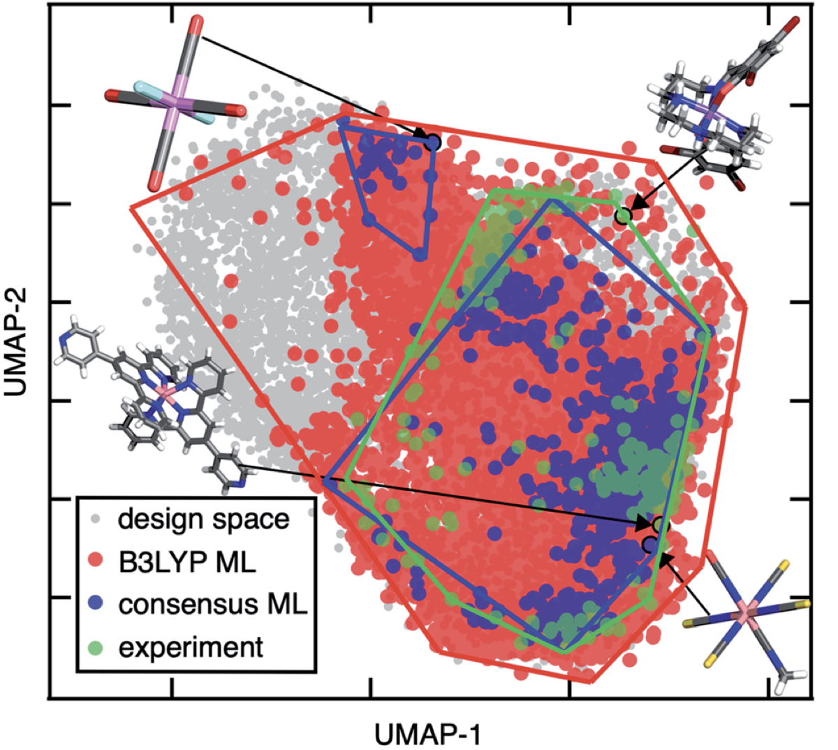
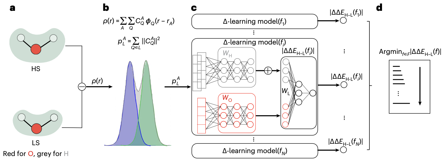
Navigating through the zoo of density functional.- The consensus approach mentioned above, though practically useful, would loose the strength of quantum chemistry, where multiple properties can be derived at once (e.g., with electron density). Inspired by modern scheme of recommendation in Spotify and Tiktok, Duan et al. recently developed a density functional recommender, which is native to the current HTC. For every single systems, this density functional recommender recommends a functional that is expected to yield the lowest error compared to the reference (e.g., experiment). Their recommender approach yields a mean absolute error of 2.1 kcal/mol, outperforming the use of any single functional in the HTC for discovering spin-crossover compounds, which are particularly sensitive to the choise of functional. Due to the use of electron density as underlying representation for their models, the recommender is transferable to out-of-distribution experimental data and molecules of completely different coordination chemistry.

Outlook

Quantum chemistry lies in the core of how people understand chemical reactions, which forms the world in which we live. Most of the pain in quantum chemistry can be attributed to the curse of dimensionality, where ML has proven to be useful to address. ML integration in quantum chemistry is a young, yet rising direction, with the potential to uncover the understanding to more complicated and large-scale chemical behavior that are both difficult to simulate in cloud and wet lab. It is an interdisciplinary field that welcomes knowledge and contribution from chemistry, physics, computer science, applied math, and more. It also welcomes you.