Author(s): Tianfan Fu is Postdoc at Computer Science Department at UIUC, supervised by Prof. Jimeng Sun. He obtained PhD degree from the Department of Computational Science and Engineering at Georgia Institute of Technology in 2023. He received his B.S. and M.S. degree at Department of Computer Science and Engineering from Shanghai Jiao Tong University in 2015 and 2018, respectively. He will join Rensselaer Polytechnic Institute (RPI) Computer Science Department as a tenure-track assistant professor in January 2024.

Motivation and Introduction

Sequential decision-making problem is a fundamental problem in many scientific real-world applications. For example, molecule optimization is a fundamental problem in pharmaceutical and material science. In pharmaceutical science, the goal is to generate a drug molecule that could bind to the target protein and inhibit the target protein to treat human diseases. In material science, the goal is to generate a material molecule with well-banded structures. It targets generating molecules with desirable properties and typically grows a molecule by adding a basic building block at one step; at each step, we need to decide how to grow a molecule (at which position and what to add).

Reinforcement Learning

Reinforcement learning, one of the most active research areas in artificial intelligence, is a computational approach to learning whereby an agent tries to maximize the total reward it receives when interacting with a complex, stochastic environment. Next, we formulate the general reinforcement learning algorithm. For ease of following, we list the mathematical notations in Table 1. | Notations | Explanation | | — | — | | \(\mathcal{S}\) | state space | | \(s^{t} \in \mathcal{S}\) | state at the \(t\)-th step of Markov decision process (MDP) | | \(\mathcal{A}\) | action space | | \(a \in \mathcal{A}\) | action | | \(R\) | reward function | | \(\pi_{\theta}(a|s)\) | policy network, given the state \(s\), predict the action \(a\) | | \(\theta\) | learnable parameter of policy network | | \(\mathcal{L}\) | objective function |

Table 1: Mathematical notations and their explanations.

Markov Decision Process

Reinforcement learning formulates the sequential decision-making problem as a Markov decision process (MDP). Markov decision process is a stochastic process that assumes given the current state, the future state does not rely on the historical state, which is also known as Markov property. That is to say, the Markov decision process satisfies Markov property, which is defined as \(p(s^{t+1}|s^{t}, s^{t-1}, s^{t-2}, \cdots, s^{1}) = p(s^{t+1}|s^{t}), \tag{1}\) where the state at the time \(t\) is denoted \(s^t\).

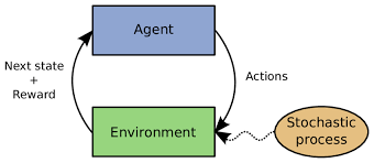
Figure 1: Markov decision process (MDP).

Then we describe the basic components of the Markov decision process. For ease of following, we list the mathematical notations in Table 1. Figure 1 illustrate the Markov decision process.

• State space. State space (denoted \(\mathcal{S}\)) incorporates all the possible states. Each time step corresponds to a state. The state at the time \(t\) is denoted \(s^t \in \mathcal{S}\).

• Action space. Action space specifies the set of all the possible actions, and the action space at time \(t\) is denoted \(\mathcal{A}_t\).

• Agent (typically a machine learning model). At the time \(t\), the agent takes the state \(s^t\) as the input and generates the action \(a^t\) from action space \(\mathcal{A}_t\). The process is denoted \(a_t \sim \pi_{\theta}(\cdot | s^t)\), \(\theta\) is the learnable parameter of the RL agent. \(\pi_{\theta}\) is also known as policy network or policy model.

• State transition dynamics. The action is performed on the state, and then the system jumps into the next state, which is denoted \(s^{t+1} \xleftarrow[]{} f(s^t, a^t)\) or \(s^{t+1} \sim f(s^t, a^t)\). The state transition \(f\) can be either deterministic or stochastic.

• Reward function. Given the state, the system would receive the reward \(r(s^t)\) from the environment, where \(r(\cdot)\) is called the reward function. The reward function takes a state as the input and yields a scalar reward. It is not differentiable concerning the state and can be seen as a black-box function.

The goal is to learn an agent that takes optimal policy and receives the maximum expected reward. The objective function can be written as \(\mathcal{L}(\theta) = \sum_{t=1}^{\infty}\mathbb{E}_{\pi_{\theta}(a^t | s^t)} [R(s^t)].\tag{2}\) The objective function is not differentiable with parameter \(\theta\). Thus, we resort to policy gradient (also known as policy learning) to optimize the objective.

Policy Gradient

Optimizing the objective function in reinforcement learning can be essentially generalized to the following optimization problem: \(\underset{\theta}{\arg\max}\ \mathcal{L}(\theta) = \mathbb{E}_{\pi_{\theta}(x)}\big[R(x)\big],\tag{3}\) where reward function \(R(x)\) is a black-box function that is not differentiable to \(x\). \(\pi_{\theta}(x)\) is a probability distribution over \(x\) and parameterized by \(\theta\), which is differentiable with respect to both \(x\) and \(\theta\). \(\theta\) is the parameter of interest. The gradient of the objective function is not analytically tractable. Policy gradient is used to estimate a gradient of the objective function.

Then the gradient of the objective function concerning \(\theta\) can be expanded as

\[\begin{aligned} \nabla_{\theta} \mathcal{L}(\theta) & = \nabla_{\theta} \mathbb{E}_{\pi_{\theta}(x)}[R(x)] \\ & = \nabla_{\theta} \int \pi_{\theta}(x) R(x) dx \\ & = \int \nabla_{\theta} \pi_{\theta}(x) R(x) dx \\ & = \int \pi_{\theta}(x) \frac{\nabla_{\theta} \pi_{\theta}(x)}{\pi_{\theta}(x)} R(x) dx \\ & = \int \pi_{\theta}(x) \nabla_{\theta} \log \pi_{\theta}(x) R(x) dx \\ & = \mathbb{E}_{\pi_{\theta}(x)} \big[\nabla_{\theta} \log \pi_{\theta}(x) R(x)\big] \end{aligned}\tag{4}\]

where “log-derivative trick” is applied in the fourth equality, we have \(\begin{aligned} \nabla \pi_{\theta}(x) = \pi_{\theta}(x) \frac{\nabla_{\theta} \pi_{\theta}(x)}{\pi_{\theta}(x)} = \pi_{\theta}(x) \nabla_{\theta} \log \pi_{\theta}(x). \\ \end{aligned}\tag{5}\) Then, the unbiased estimator for the gradient of \(\mathcal{L}(\theta)\) concerning parameters \(\theta\) can be obtained. Stochastic gradient ascent is used to maximize the objective function concerning \(\theta\) based on the noisy gradient. Please refer to [1] for a description of the policy gradient.

Successful Applications of Reinforcement Learning in Scientific Discovery

In this section, we exemplify reinforcement learning with two real-world applications of scientific research across various disciplines, including molecule optimization and retrosynthesis planning.

Molecular Optimization

Molecular optimization, also known as molecule design or molecule discovery, is a fundamental problem in many disciplines such as material science [2] and pharmaceutical science [3]. The goal is to produce novel molecules with desirable properties. For example, in material science, we want to design material molecules with well-banded structures; in drug discovery, we want drug molecules that can bind tightly to the target protein (the cause of human diseases).

We use graph convolutional policy network (GCPN) [4] as an example. Next, we elaborate on the basic RL components in GCPN.

• State. It uses the partially generated molecular graph as the state. The state space is the whole chemical space. The initial state is a carbon atom.

• Action space. In each step, GCPN has four types of actions, defined as follows.

  1. selecting the first atom from the atoms in the current molecular graph. It is performed as a multi-category classification task.

  2. selecting the second atom, which can be either from the current molecular graph or a new atom in the vocabulary. It is also a multi-category classification task.

  3. selecting the type of bond that connects the first and second atoms. There are totally four bond types, single bond, double bond, triple bond, and aromatic bond (in the aromatic ring).

  4. determining whether to stop, which can be viewed as a binary classification task.

• Agent. GCPN uses graph convolutional network (GCN) [5] as the neural architecture. GCN takes a (incomplete) molecular graph as the input feature and produces the node embeddings for all the nodes. It leverages four GCNs for the four actions above.

  1. GCN first generates the node embeddings of all the nodes, then uses a multiple layer perception (MLP) to all the embeddings (followed by a softmax activation) and generates a categorical distribution.

  2. GCN first generates the node embeddings of all the nodes, and we also generate an embedding for each atom in the vocabulary. Then it uses a multiple-layer perception (MLP) to produce a categorical distribution based on all the nodes’ embeddings (followed by a softmax activation).

  3. GCN first generates the node embeddings of all the nodes, then we aggregate all the node embeddings into a graph-level embedding, followed by an MLP to perform 4-category classification.

  4. GCN first generates the node embeddings of all the nodes, then we aggregate all the node embeddings into a graph-level embedding, followed by an MLP to perform binary classification.

• State transition dynamics. Here the state transition is deterministic, i.e., connecting two atoms with the predicted bond type and then determining whether to stop.

• Reward function. In molecule optimization, the goal is to maximize the property of the generated molecule, so we evaluate the molecular property of the partially generated molecular graph (i.e., current state) and use it as the reward function.

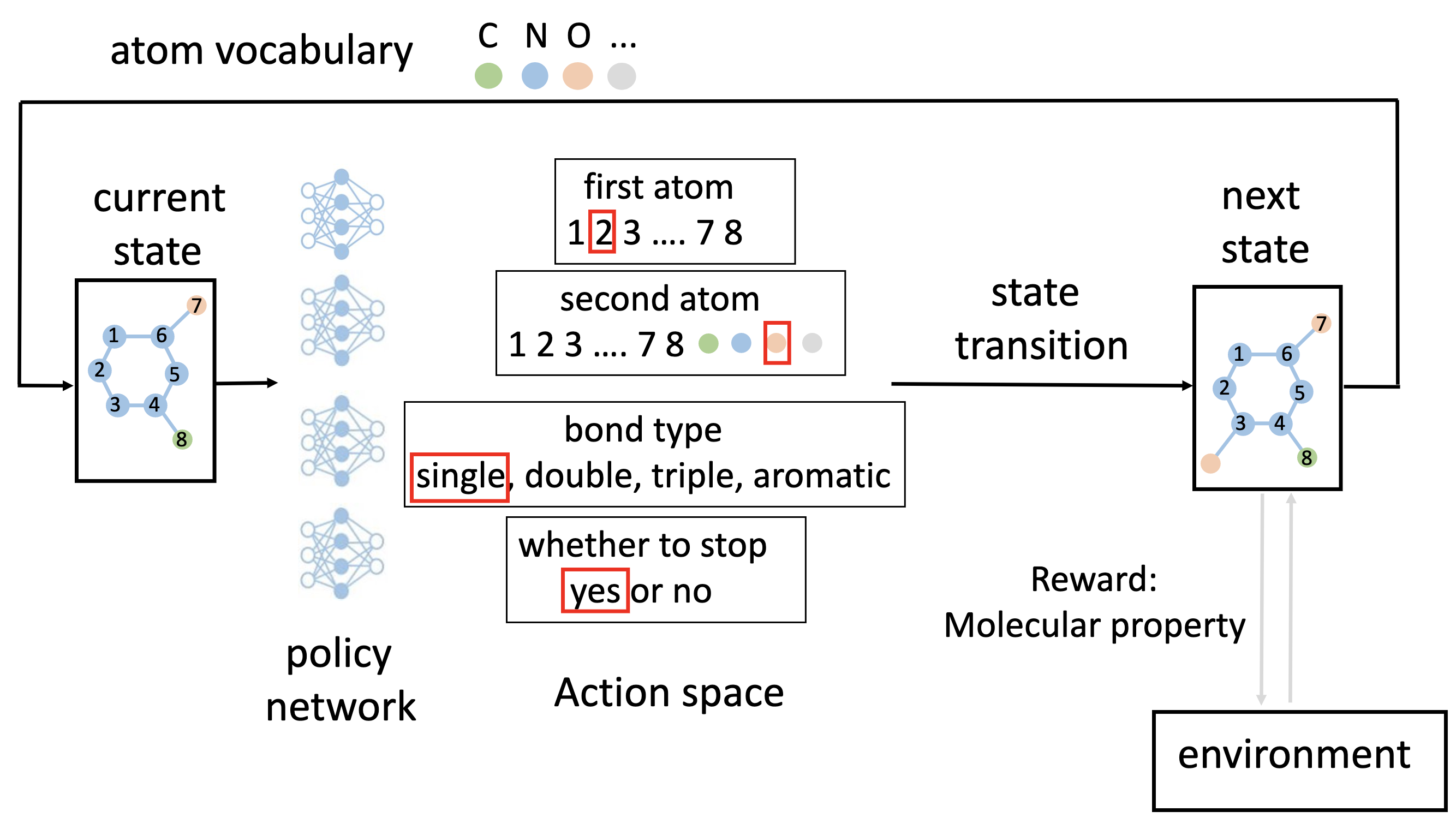
Figure 2: Illustration of graph convolutional policy network (GCPN) for molecular optimization.

Other variants have also been validated to be effective in molecular optimization, such as REINVENT [6] and reinforced genetic algorithm (RGA) [7]. Specifically, REINVENT [6] formulates molecular string as a sequential decision-making problem, where we need to decide which token to add in each step. It uses SMILES string[^1] as molecular representation and leverage gated recurrent unit (GRU) [8] (a popular variant of recurrent neural network (RNN)) as the agent. In each step, the action is to add a token. The state transition is deterministic. The reward function is the molecular property of the current state (partially generated SMILES string). On the other hand, reinforced genetic algorithm (RGA) [7] formulates the genetic algorithm as a Markov decision process, where the population in each generation is regarded as the state; the action is to select the candidate to be mutated or crossover; the state transition is deterministic; the reward is the molecular property.

Retrosynthesis Prediction

Retrosynthesis prediction forecasts the reactants given the products. It is a key step in drug manufacturing. In small-molecule drug design, scientists or machine learning models usually design the drug molecule with desirable pharmaceutical properties. Then they want to know how to synthesize these chemical compounds using a series of chemical reactions.

The machine learning model would generate reactants, which can be formulated as a Markov decision process. We discuss the paper [9]. The whole process is illustrated in Figure 3. Then we show the basic components of MDP in retrosynthesis prediction.

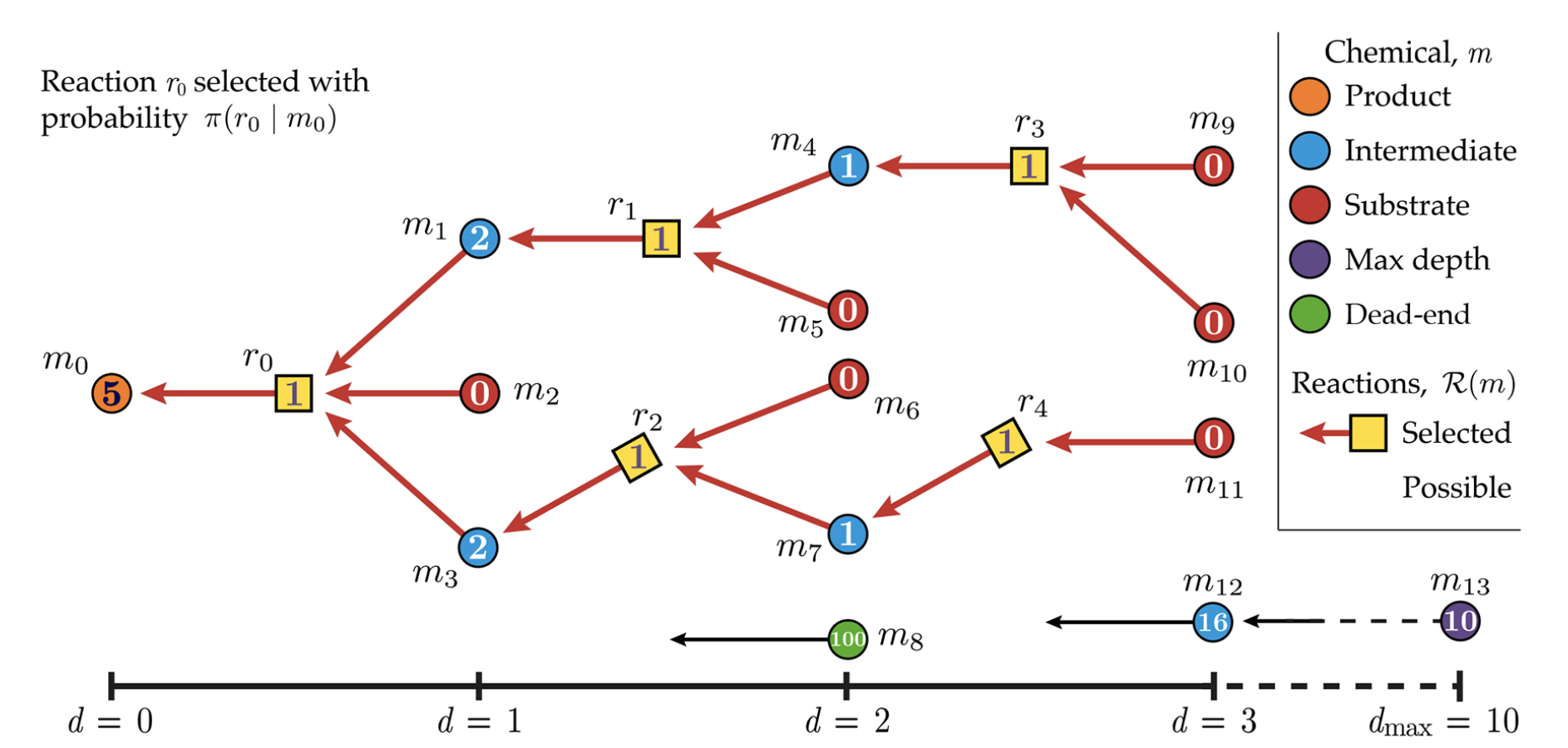
Figure 3: Illustration of reinforcement learning for retrosynthesis prediction. In this step, we use an agent (policy network) to select the action. Then after conducting the action, we jump into the next state. The reward is designed to measure the complexity and accessibility of the synthetic route. The maximum depth is set to 10. Dead-end represents the molecules that cannot be synthesized. “0” within the circle means the chemical compound is in the purchasable database.

• State. In each step, the state is all the reactants that could generate the target product. For example, in Figure 3, if we choose the \(r_0\), the state is \(M = (m_1, m_2,m _3)\).

• Action space. We maintain a database of chemical reaction templates. Given the target molecule to be synthesized, we enumerate all the templates and keep all the possible combinations \(r\) as the action space.

• Agent. Agent (policy network) is a multiple-layer perception (MLP). It can be written as \(\pi(r|(M,d))\). It takes the concatenation of the molecular extended-connectivity fingerprint (ECFP) fingerprint of reactants \(M\) and the depth (\(d\) in Figure 3 as the input and predicts the probability of \(\pi(r|m_0)\) (normalized over all the possible actions).

• State transition dynamics. The state transition is deterministic. Since we use reaction templates, the reactant (precursor) is unique once we select the action.

• Reward function. The reward function is a composite function that considers the penalty of the depth \(d\) and the accessibility of the reactant. Deeper depth means more complex the synthetic route and is less desirable. We have a database of all the purchasable chemical compounds to measure the accessibility of the reactant. When the reactant is in the database, we assign a high reward value.

How to apply reinforcement learning to scientific problem

We need to consider the following questions when applying reinforcement learning.

• Can the problem be formulated as a sequential decision-making problem? If the answer is not, deploying reinforcement learning to your problem is hard.

• What is state and state space? For example, in molecular design, the state could be the partially generated molecular graph.

• What are action and action space? For example, in molecular design, the action could be adding a new atom and connecting it to an existing node in the partially generated molecular graph.

• How to design the agent (i.e., policy network) that predicts the action given the state?

• How is the state transferred? That is, given the state, an action is performed, what is the next state? For example, in molecular design, the state transition is deterministic. That is, once we select the first and second atoms and the bond type, we can determine generated molecule without stochasticity.

• What is the reward function? For example, in molecular design, the reward function can be the pharmaceutical property of the generated molecules that we want to optimize.

Learning Resources

In this section, we recommend publicly available learning resources that help the audience acquire RL and deploy RL to their own problem.

• Prerequisite: A basic knowledge on machine learning is necessary; also, most of the recent progress in reinforcement learning is combined with deep learning, so it would be great if the reader had a background in deep learning.

• Textbook: “Reinforcement learning: An introduction “ [10]. This book provides a clear and simple account of the key ideas and algorithms of reinforcement learning. Their discussion ranges from the history of the field’s intellectual foundations to the most recent developments and applications.

• Courses: We refer a highly practical course named “Reinforcement Learning beginner to master – AI in Python”. Also, another reinforcement learning course is from Udacity. https://www.mltut.com/best-deep-reinforcement-learning-courses/ recommend 10 best reinforcement learning courses.

• Survey: traditional reinforcement learning (before deep learning era, written in 1996) [11], deep reinforcement learning (more recent, written in 2017) [12].

• Tutorial: we recommend [13].

• Benchmark: [14] benchmarks a series of popular downstream reinforcement learning applications such as cart-pole swing-up, 3D humanoid locomotion, etc. The code is open-sourced at https://github.com/rllab/rllab.

• Codebase: OpenAI Baselines is a set of high-quality implementations of reinforcement learning algorithms. These algorithms will make it easier for the research community to replicate, refine, and identify new ideas. It is available at https://github.com/openai/baselines.git.

References

[1] Sham M Kakade. A natural policy gradient. Advances in neural information processing systems, 14, 2001.

[2] Ruimin Zhou, Zhaoyan Jiang, Chen Yang, Jianwei Yu, Jirui Feng, Muhammad Abdullah Adil, Dan Deng, Wenjun Zou, Jianqi Zhang, Kun Lu, et al. All-small-molecule organic solar cells with over 14% efficiency by optimizing hierarchical morphologies. Nature communications, 10(1):1–9, 2019.

[3] David C Swinney and Jason Anthony. How were new medicines discovered? Nature reviews Drug discovery, 10(7):507–519, 2011.

[4] Jiaxuan You, Bowen Liu, Zhitao Ying, Vijay Pande, and Jure Leskovec. Graph convolutional policy network for goal-directed molecular graph generation. In Advances in neural information processing systems, 2018.

[5] Thomas N Kipf and Max Welling. Semi-supervised classification with graph convolutional networks. The International Conference on Learning Representations (ICLR), 2016.

[6] Marcus Olivecrona, Thomas Blaschke, Ola Engkvist, and Hongming Chen. Molecular de-novo design through deep reinforcement learning. Journal of cheminformatics, 9(1):48, 2017.

[7] Tianfan Fu, Wenhao Gao, Connor W Coley, and Jimeng Sun. Reinforced genetic algorithm for structure-based drug design. In Annual Conference on Neural Information Processing Systems (NeurIPS), 2022.

[8] Kyunghyun Cho, Bart van Merrienboer, Caglar Gulcehre, Dzmitry Bahdanau, Fethi Bougares, Holger Schwenk, and Yoshua Bengio. Learning phrase representations using RNN Encoder–Decoder for statistical machine translation. In Proceedings of the 2014 Conference on Empirical Methods in Natural Language Processing (EMNLP), pages 1724–1734, Stroudsburg, PA, USA, 2014. Association for Computational Linguistics.

[9] John S Schreck, Connor W Coley, and Kyle JM Bishop. Learning retrosynthetic planning through simulated experience. ACS central science, 5(6):970–981, 2019.

[10] Richard S Sutton and Andrew G Barto. Reinforcement learning: An introduction. MIT press, 2018.

[11] Leslie Pack Kaelbling, Michael L Littman, and Andrew W Moore. Reinforcement learning: A survey. Journal of artificial intelligence research, 4:237–285, 1996.

[12] Kai Arulkumaran, Marc Peter Deisenroth, Miles Brundage, and Anil Anthony Bharath. Deep reinforcement learning: A brief survey. IEEE Signal Processing Magazine, 34(6):26–38, 2017.

[13] Sergey Levine. Reinforcement learning and control as probabilistic inference: Tutorial and review. arXiv preprint arXiv:1805.00909, 2018.

[14] Yan Duan, Xi Chen, Rein Houthooft, John Schulman, and Pieter Abbeel. Benchmarking deep reinforcement learning for continuous control. In International conference on machine learning, pages 1329–1338. PMLR, 2016.